Create Dynamic Rows for an Amortization Schedule with Power Query

Sometimes in Excel, we want to use formulas to compute row values, but, the number of rows is dynamic and changes periodically. For example, let’s say we want to create an amortization schedule and use it for a variety of loans. Some loans are paid in 36 months, some in 120 months, and some in 360 months. So, we need anywhere from 36 rows to 360 rows. Or, possibly less, or, perhaps more … it just depends on the current loan term. The point here is that number of rows is variable.

Traditionally, a common solution was to create more rows of formulas than you’d ever need, and then use some technique to hide the formulas in rows that aren’t used for the current schedule. For example, we could use conditional formatting, manually hide rows, use outline groups, or use dynamic named ranges for printing.

However, Power Query provides another option. You see, Power Query can create a dynamic number of rows based on your input. Although this technique can be used in a variety of ways, I’ll illustrate the approach with a basic loan amortization schedule.

Objective

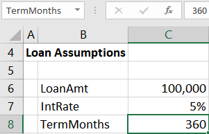
For example, let’s say we enter these basic loan assumptions:

Now we want an amortization schedule that displays one row for each month. If the loan term was 360 months we’d want 360 rows, and so on.

We could do this by writing formulas in the maximum number of rows needed for any loan. So, if the max mortgage term was 30 years, we would write formulas in 360 monthly rows. Then, we would use some technique to hide the excess formulas for shorter loan terms. The benefit of this approach is that formulas automatically recalculate, so, you enter the assumptions and you are done with the math. The disadvantage is that for shorter loan terms, you’ll have a bunch of extra formulas to manage. You may have to hide them, delete them, conditionally format them, or use some other method. And then, if you get a longer term, like a 40 year mortgage, then you have to fill formulas down into additional rows. Basically, you are manually managing the number of rows to match each loan term.

Alternatively, we could use Power Query to dynamically provide the correct number of rows based on the loan term. The advantage is that it provides the exact number of rows needed, so there is no need to hide rows or fill formulas down manually. The disadvantage is you have to manually right-click > Refresh the amortization table.

So, with that background in place, let’s walk through the details for using Power Query to dynamically generate the number of rows needed based on the loan term.

Details

We’ll use these steps to accomplish our goal.

• Retrieve the loan term
• Create a dynamic list of periods
• Write the Excel formulas
• Add the total row

Let’s get to it.

Note: The steps below are presented with Excel for Windows 2016. If you are using a different version of Excel, please note that the features presented may not be available or you may need to download and install the Power Query Add-in.

Retrieve the loan term

First, we need to get the loan term in months into Power Query. One fairly quick way to do this is to use a named range. We basically assign a defined name to the input cell that stores the loan term. One way to do that is to select the input cell and then enter the desired name into the Name Box (the little box to the left of the formula bar). Our name will be TermMonths so, we select the cell that stores the loan term (12, 36, 120, etc.) and then type the name TermMonths into the Name Box and hit Enter.

We can confirm our cell is named by selecting the cell and viewing the Name Box, as shown below.

To bring the value in the TermMonths named cell into Power Query, we select the named input cell and click the Data > From Table/Range button. The value in the cell is displayed in the editor. Now, we will change the query name by using the Name field in the query editor. We simply change the Query Name to a preferred name, such as TermMonths. The next step will be a bit easier if we avoid spaces, so, I went with TermMonths without any spaces as shown below.

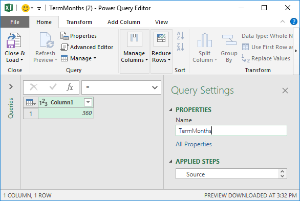
The final step is to Drill Down so that we can easily reference this value in another query. To do this, we right-click the value 360 and select Drill Down, the results of which are shown below.

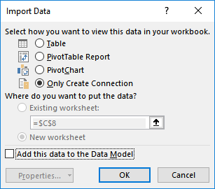
With this complete, we can now select Close & Load To, and then select Only Create Connection as shown below.

At this point, we have a query that retrieves the user-entered term in months. So far so good, now it is time to create the dynamic list of periods.

Create a dynamic list of periods

We begin by opening up a blank query. To do this, we select Data > Get Data > From Other Sources > Blank Query.

We get a new empty query, as shown below.

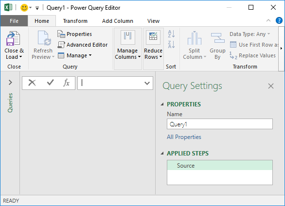
Now, assuming we named our previous Query TermMonths, we define the Source step by entering the following formula:

={1..TermMonths}

This is shown below.

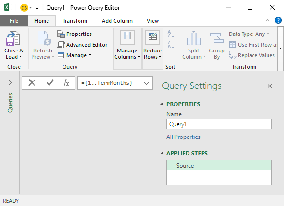
Now for the moment of truth … we hit Enter after writing the formula and … BAM! Excel creates a list of numbers from 1 to the number of months, as shown below.

The great part about this is that this list will dynamically update when a user enters a different value in Excel and then refreshes the query results table.

Wait, what just happened here? Well, the curly braces { } tell Excel to create a List. The two dots tell Excel to fill in the values between the start point, 1, and the end point, the value provided by the TermMonths query. As you might expect, as the TermMonths number changes so does the list and resulting number of rows.

We rename the query to Period as shown below.

We send the results back to Excel by selecting Home > Close and Load To, and select Table as shown below.

And the list of periods appears in the specified location, as shown below.

Now, a user can enter a new term, and then right-click > Refresh to update the results table. Nice 🙂

All that remains is to write the Excel formulas.

Write the Excel formulas

We’ll break this part into a few steps. First, we need to know the monthly payment amount.

Compute the Monthly Payment Amount

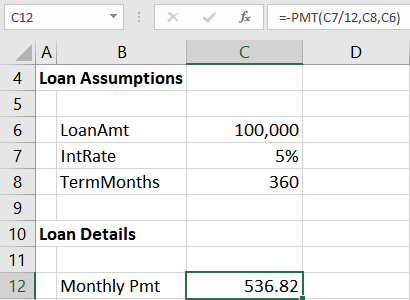
We’ll use Excel’s PMT function to compute the monthly payment amount. Assuming the annual interest rate is stored in C7, the loan term is stored in C8, and the loan amount in C6, the formula would be:

=-PMT(C7/12, C8, C6)

This is shown in the screenshot below.

Note: if you’d like more detail on the PMT function, check out this blog post.

Next, we need to create new columns in the results table.

Add New Column Headers

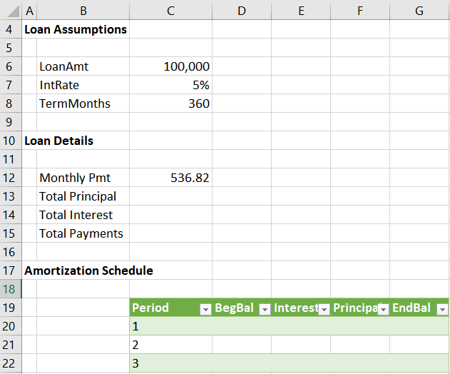
We’d like our amortization schedule to include the following columns:

• Period
• BegBal
• Interest
• Principal
• EndBal

We already have the first column, Period, created by Power Query. So, we just need to add the others. To do this, we type the new column label in the cell right of the existing label and the table auto-expands to include it.

For example, we enter the next column label BegBal immediately right of the existing Period label, and the table expands as shown below.

We do this for all desired columns, as shown below.

Now we need to write the formulas that compute the amounts for each column.

Write Corresponding Formulas

There are many variations of formulas that will compute these amounts, so, these formulas provide but one solution. Many others exist.

We enter the following formulas into the Period 1 row for each column. As we hit Enter after writing each, Excel auto-fills the formula down.

• BegBal = IF(ISTEXT(H19),$C$6,H19)
• Payment = $C$12
• Interest = -IPMT($C$7/12,[@Period],TermMonths,$C$6)
• Principal = [@Payment]-[@Interest]
• EndBal = [@BegBal]-[@Principal]

Yay! We now have a basic amortization schedule, as shown below.

With this complete, we just need to compute a few totals.

Add the total row

To compute the total interest and total principal provided in the amortization schedule, we just need to turn on the table’s total row. We do this by selecting any cell in the table and then checking the Table Tools > Total Row check box.

Then, in the new total row that appears at the bottom of the table, we select the cell in the Interest column and use the drop-down to pick Sum. We do the same for the Principal column.

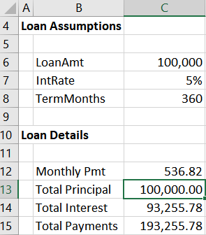
Then, we retrieve the values into any desired cell by typing = and then pointing to the corresponding total row cell. For example, we retrieved the Total Principal and Total Interest values into cells C13 and C14 below.

Now, when we need to perform an update, we just enter the three loan assumptions, and right-click > Refresh the results table. We have the exact number of rows needed.

Note: Power Query doesn’t operate like Excel formulas, and so the table won’t expand or shrink the number of rows until you right-click > Refresh.

My goal here was to talk about how Power Query can dynamically adjust the number of rows in a table. The illustration I used to demonstrate this was an amortization schedule. If you have any other fun Power Query tricks, please share by posting a comment below … thanks!

Sample File:

• PQAmort.xlsx
• Daily Interest.xlsx