Moving, Rolling, and Trailing Averages

The terms Moving, Rolling, and Trailing are commonly used to describe the same calculation idea…that we want to operate on the previous say 3, 6, or 12 data rows. In this post, we’ll allow the user to define the number of rows to include and use the OFFSET function to dynamically define the desired range.

Objective

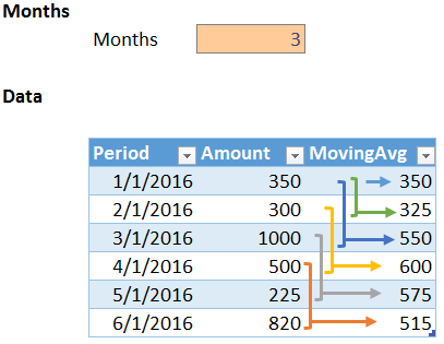
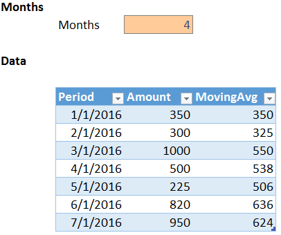
Before we get too far, let’s be clear about our objective. We want to allow the user to enter the number of rows to include. We want to write a formula that computes the average of the desired number of rows. This is illustrated below.

We also want to ensure that as we add new rows to the table in future periods, we don’t need to update our formula. One way to accomplish this is with the OFFSET function.

OFFSET

The volatile OFFSET function allows us to define a range via its arguments. The syntax follows.

OFFSET(reference, rows, columns, [height], [width])

Where:

• reference is the starting point
• rows is the number of rows down (+), or up (-), to move the starting point
• columns is the number of columns right (+), or left (-), to move the starting point
• [height] is the total number of rows in the desired range
• [width] is the total number of columns in the desired range

For example, if we wanted to start at A10, move down 3 rows and move right 1 column, we could use the following function.

OFFSET(A10,3,1)

If we wanted to start at A10, move up 2 rows, move right 0 columns, set the total number of rows to 3, and the total number of columns to 1, we could use the following function.

OFFSET(A10,-2,0,3,1)

The OFFSET function returns a range reference, so, to do something with it, such as find the average, we need to wrap the desired function around the OFFSET. For example, to find the average of the range returned by the OFFSET function, we could use the following formula.

=AVERAGE(OFFSET(A10,-2,0,3,1))

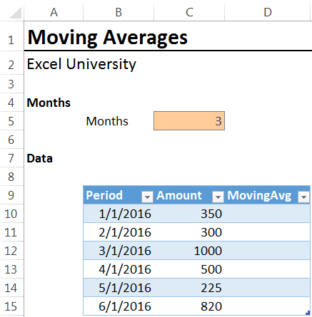
Now that we have the basic logic down, let’s use this with a table and allow the user to store the number of periods in a cell. We begin by converting the ordinary data range into a table with the Insert > Table icon. Next, we want to write a formula to populate the MovingAvg column.

Instead of using an A1-style reference, such as A10, we reference the amount cell for the current row with a structured table reference. When you click the cell, Excel inserts the correct table reference, such as [@Amount]. For example, we could write the following formula into the first table row.

=AVERAGE(OFFSET([@Amount],-2,0,3,1))

However, that would fix the number of months within the formula, and, since we want to make it easy for the user to change the number of months in our average, we store the months value in cell C5, and then update our formula as follows.

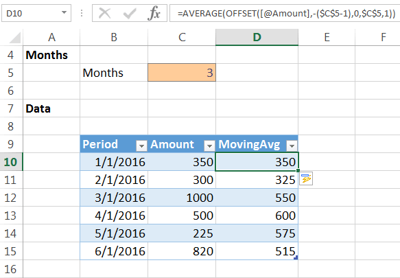
=AVERAGE(OFFSET([@Amount],-($C$5-1),0,$C$5,1))

We hit enter and…yes…it worked!

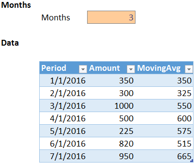
When we add another table row, Excel automatically fills the MovingAvg formula down, as shown below.

And, the user can change the number of months, as shown below.

Optional Enhancement

Now, there is one optional enhancement to discuss. With the formula above, the OFFSET function creates a range for the first few table rows that may extend above the table. For example, the formula in the first table row begins a few rows above the table. As long as there are enough non-numeric cells above the Amount column, there is no issue. However, we can modify our formula so that the range returned by the OFFSET function stays within the table. This is done by computing the row number with the ROWS function, and then returning the MIN between that number of rows and the desired number of rows. The updated formula is shown below for reference, and is also included in the sample Excel file.

=AVERAGE(OFFSET([@Amount],
-MIN($C$5-1,(ROW()-ROW(Table1[#Headers]))-1),
0,
MIN($C$5,ROW()-ROW(Table1[#Headers])),
1))

This is great, because now the user can specify the desired number of months, and our moving average formula will update accordingly. Plus, as new data rows are added Excel fills the formula down for us since we used a table.

INDEX

Now that we have the basic idea down, let’s use an alternative to the volatile OFFSET function, the non-volatile INDEX function. The basic idea here is that the OFFSET function is volatile, which means Excel recalculates it anytime any value has changed, whereas, non-volatile functions are recalculated when precedent cells have changed. In summary, for small workbooks either function would probably be just fine, however, in large workbooks it is best practice to avoid volatile functions when possible. That is why the INDEX function is typically preferred.

The basic idea here is that we use the range operator to define the range, and the first side is the amount value in the current row. Then we use the INDEX function to return a reference to the cell that is say two rows above that cell. This can be accomplished with the following INDEX function.

=AVERAGE([@Amount]:INDEX([Amount],MAX((ROW()-ROW(Table1[#Headers]))-($C$5-1),1),1))

Where:

• [@Amount] is the first side of the range, the current row Amount cell
• INDEX([Amount],MAX((ROW()-ROW(Table1[#Headers]))-($C$5-1),1),1) returns the second side of the range operator
• Where:
  • [Amount] is the entire Amount column
  • MAX((ROW()-ROW(Table1[#Headers]))-($C$5-1),1) returns the number of rows above
  • 1 means the first column in the range

If you have any alternatives or preferred formulas, please share by posting a comment below…thanks!

Additional Resources

• Sample File
• INDEX posts