Sum Last N Columns

If you have a data table that is updated frequently, for example, a new column is added each month, you may want to find the sum of the last three columns. But, you don’t want to rewrite your formula each time you add a new column. Fortunately, you can accomplish this task with two lookup functions, INDEX and COLUMNS.

Objective

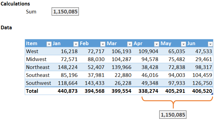
Let’s be clear about our objectives. We want to write a formula that operates on the last three columns. We do not want to modify the formula each time a new column is added. For example, the formula below computes the sum of the last three table columns, Apr, May, and Jun.

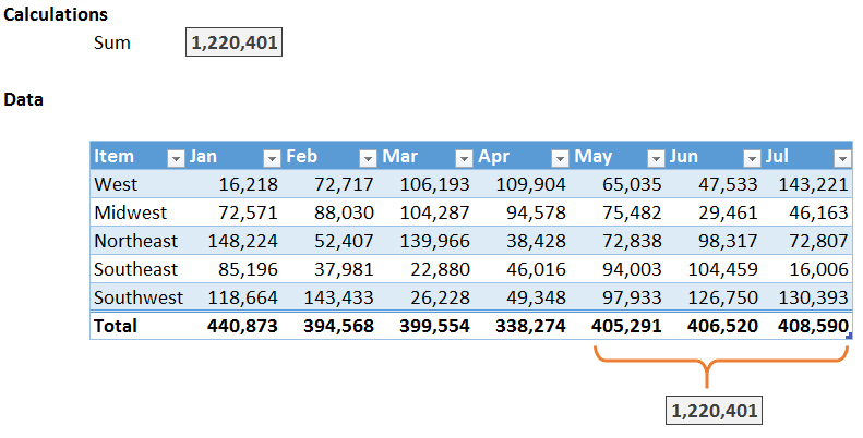
Next month, we’ll add a new Jul column, and, we want our formula to automatically sum the last three columns in the table, May, Jun, and Jul as shown below.

Excel’s COLUMNS and INDEX functions can be used as arguments in the SUM function so that the formula will automatically sum the last three columns in the table, even as new columns are added each month. Let’s walk through the details of the formula now.

Details

The basic formula begins with a standard SUM function. Assuming our table is named Table1, we could add up all of the cells in the table with the following formula.

=SUM(Table1)

But…we don’t want to add up all of the cells in the table, we only want to add up the cells in the final three columns. So, let’s explore the INDEX function to narrow down the table reference.

If we wanted to add up the cells in the 2nd table column, we could use INDEX to narrow down the reference as follows.

=SUM(INDEX(Table1,0,2))

Where:

• Table1 is the entire table range
• 0 means we want to include all rows within the range
• 2 means we want to include the 2nd column within the range

Let’s say that instead of adding up the 2nd column, we want to add up the last column. Rather than expressing the argument with an integer value such as 2, we want Excel to dynamically figure out the last column number. This brings us to the COLUMNS function which returns the number of columns within a range. For example, the following formula will return the number of columns in our table, which happens to be 8 at the moment.

=COLUMNS(Table1)

As the number of columns in the table changes, the COLUMNS function updates it result as well, from 8, to 9, to 10, and so on.

If we wanted to add up the last column of the table, column 8, we could use the following formula.

=SUM(INDEX(Table1,0,COLUMNS(Table1)))

Where:

• Table1 is the table reference
• 0 means we want to include all rows
• COLUMNS(Table1) means we want to include the last column

But…we don’t want to sum the final column, we want to sum the final three columns. No problem, we can just include another INDEX function. Essentially, we’ll use one INDEX function to specify the first column in the desired range (column 6), and another INDEX function to specify the last column in the range (column 8).

You know that you can use the range operator (:) to specify a range using cell references, such as A1:B10. You can also use the range operator with two INDEX functions, such as INDEX(…):INDEX(…). In the formula below, the first INDEX function references the May column (8-2=6) and the second INDEX function references the Jul column (column 8).

=SUM(INDEX(Table1,0,COLUMNS(Table1)-2):INDEX(Table1,0,COLUMNS(Table1)))

Where:

• INDEX(Table1,0,COLUMNS(Table1)-2 references the May column
• INDEX(Table1,0,COLUMNS(Table1) references the Jul column

Since the COLUMNS function updates anytime a new column is added, the formula will return the SUM of the last three columns of the table. If you wanted to sum the last 6 columns, you would simply subtract 5 instead of 2 from the first INDEX function’s column argument. If you wanted the last 12, you’d subtract 11, and so on.

If you have any other approaches to summing the final three table columns, please share by posting a comment below…thanks!

Note

• This technique can also be used to sum the last n rows of data…just use the ROWS function as the rows argument…such as INDEX(Table1,ROWS(Table1),0)

Additional Resources

• Sample Excel File
• INDEX function posts