Highlight Values Found Multiple Times

Today, we’ll highlight recurring values within a dataset in order to answer a recent question. I was asked the following “I’m trying to get it to recognize if a specific letter, like X, is in a column at least three times. What could the formula look like?” And I’ll answer that question in this post. Let’s just dive in!

Video

Step-by-step

We’ll walk through a series of three exercises to demonstrate the key elements.

Exercise 1: Exploring the COUNTIF Function

First we need to understand how to determine how many times a cell matches a specific value. We’ll use the COUNTIF function since it has been around forever and is available in just about every Excel version in use today.

Specifically, COUNTIF counts the number of cells that match the value we are seeking. It does not count the number of times the matching value is found. When each value is found within a cell only once, this is the same count. But, when the value we are seeking is found multiple times within a single cell, the count will be different. In other words, if we are looking for the letter x, and it is found two times in one cell, COUNTIF will return 1 because it has been found in that cell. COUNTIF is counting cells. I provide other formula variations below in case you need different logic.

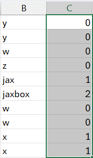
Let’s provide an illustration. Consider the range below.

We would like to count the number of times a given letter, say x, is found within the range. We type the letter we are trying to find into a cell, like C6, and then write the following formula in a cell like C8:

=COUNTIF(B12:B21,C6)

This counts the number of cells within the range B12:B21 where the cell matches cell C6. In our case it returns 4 since x is the cell value for 4 cells:

So, to reiterate, this formula counts the number of cells where the cell value matches C6. Depending on what you are working on, you may want a variation.

Variations

Depending on your data and goal, you may want to make some formula adjustments. The formula above includes in the count the number of cells that match the value exactly. Like, the full cell value is equal to the value we are seeking. But you may want other counts.

Count cells with a partial match

You may want to do a partial match. This is where we want to count the cell if the value in C6 is found anywhere within the cell. In other words, it doesn’t need to be an exact match, it can be a partial match. That way, “jax” would still match when “x” is the value to find. If so, simply update the C6 argument from C6 to:

"*" & C6 & "*"

Placing the asterisk wildcard characters around the cell value tells Excel that the value in C6 can be located anywhere within the cell. We use the concatenation operator & to join the wildcards to the cell value. So the updated ‘partial match’ formula would be:

=COUNTIF(B12:B21, "*" & C6 & "*")

Count number of occurrences

If you’d like to count the number of times that the individual letter is found in all of the text in all of the cells, we can create a helper column next to the range like this:

=LEN(B12)-LEN(SUBSTITUTE(B12,$C$6,""))

We can then fill this helper column down:

And then we can just sum up the helper column values to determine the number of times that character is found within the range.

Now, what if we wanted to do this within a Table, and highlight it with conditional formatting. That leads us to the next exercise.

Exercise 2: Step up the game – Utilizing Tables and Conditional Formatting

Now that we’re familiar with the COUNTIF function, let’s explore how to use Excel Tables and Conditional Formatting to better visualize our data. If you’ve yet to make the most out of Tables, don’t worry – transforming an ordinary list into a Table is a breeze. Simply select any cell on the range and click the Insert > Table command.

To display the count of the number of matching cells in our Table, we’ll use our trusty COUNTIF function. Our List column contains the values we would like to count:

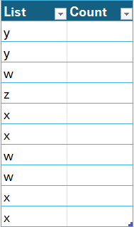
We can generate the count of the number of cells that match the value in the cell to the left by writing the following formula into the Count column:

=COUNTIF([list], [@list]) 

We hit Enter, and bam:

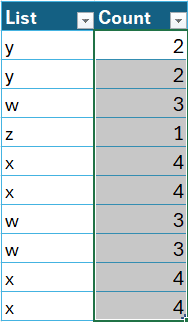
Note: since this formula is written inside the Table, we don’t need the Table name prefix in our formula. We can just use the column name.

To highlight the values that exist more than a given number of times, we can apply Conditional Formatting. Just select the entire Count column and select Home > Conditional Formatting > Highlight Cell Rules > Greater Than. In the resulting dialog, enter your desired value and formatting:

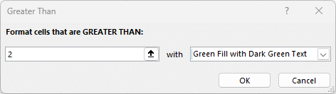
Click OK and bam:

But, what if you don’t want to have to scroll down the Table to locate the matching the cells. What if instead, you wanted to pull the values that appeared more than twice out of the Table and into a concise list? Well, that brings us to our final exercise.

Exercise 3: Beyond Basic Formatting with FILTER and UNIQUE

Now, let’s say we need a separate list of the values that appear more than 2 times. This is where we can use the FILTER and UNIQUE functions. Combining these functions, we can generate a unique, dynamic list of values that occur more than twice in our initial list. We’ll break the formula into two steps.

First, we need to understand how the FILTER function works. It returns a subset of a range. The range will be our list values, and the subset of it will be those with a count greater than 2 (or whatever number you are after).

We write the following formula:

=FILTER(Table1[List],Table1[Count]>2)

And bam:

Note: since this formula is written outside of the Table, we need to include the Table name prefix.

That formuls returns a list of the values found more than 2x. But, the result contains duplicates. We can remove the duplicates with the UNIQUE function. We simply wrap it around our existing formula like this:

=UNIQUE(FILTER(Table1[List],Table1[Count]>2))

Hit Enter, and bam:

And voilà! With these handy techniques, we can identify and highlight values that pop up multiple times in our data.

I hope this post is helpful, but if you have any follow up questions, suggestion, or alternatives, please share in the comments section below. Thanks!

Sample File

Download the sample file.

FAQ

Q: How does COUNTIF function work in Excel?

A: The COUNTIF function in Excel is used to count cells that meet a certain criterion.

Q: What are Excel Tables?

A: Excel Tables are a structured range of cells that allows for easier data management.

Q: How do I apply Conditional Formatting in an Excel table?

A: Select the cells you want to format, go to Home > Conditional Formatting > Highlight Cell Rules > and select your desired option.

Q: How does the FILTER function work in Excel?

A: The FILTER function is used to filter a range of data based on certain criteria.

Q: What does the UNIQUE function do in Excel?

A: The UNIQUE function gives a list of unique values in a range or array, eliminating any duplicates.