Dynamic Chart Title with Slicers

Here’s the situation. We have created a PivotTable and related PivotChart, and, since we are nice, we have also provided a Slicer so that the user can easily make selections. But, we’d like the report titles to dynamically update based on the selections made. As with anything in Excel, there are multiple ways to accomplish this. In this post, we’ll use a helper PivotTable.

Objective

Here is our beautiful PivotTable and related PivotChart.

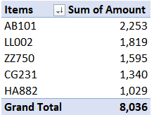
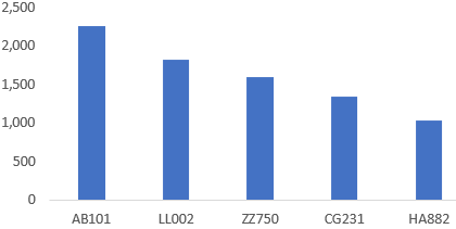
Both display sales by Item. In order for the user to be able to pick a region or regions to include in both reports, we have created a slicer, as shown below.

When the slicer is on the same worksheet as the reports, the user can easily see which regions are selected even when printed. However, the slicer may be located on a different worksheet or control several reports throughout the workbook. We’d like each report to clearly let the reader know which regions are included in the report. So, we’ll just set up a dynamic report title, something along these lines:

We’ll use dynamic report titles for the PivotTable and the PivotChart.

I’ve created a video and written narrative below that walks through the details.

Video

Narrative

We’ll work through the following steps:

• Helper PT
• Helper formula
• Pull into reports

Let’s get to it.

Helper PT

The first step is to create a helper PivotTable. The helper PivotTable has one job: display the items that the user selected in the slicer. To do this, we first create a PT based on the same data source and insert the field used for the slicer into the Columns layout area. At this point, all items in the field are displayed in the report, as shown below.

In order to have the slicer update this helper PT, we need to select the slicer and then click Slicer Tools > Report Connections. In the resulting Report Connections dialog, we check the checkbox for our helper PT, which is stored on the Settings worksheet as shown below.

Now, the slicer selections impact the helper PT as well. Since East and West are selected in the slicer, the PT is updated accordingly, shown below.

The final step is to remove the Grand Total label, which can easily be done by clicking the PivotTable Tools > Grand Totals > Off for Rows and Columns command.

Nice, the updated PT is shown below.

At this point, selections made in the slicer will be displayed in the PT. So far so good. Our next step is to create a helper column to combine the values.

Note: In this post, I’ve placed the field into the columns layout area so that the selections will appear on a single row, but, you could easily adapt the steps presented if you prefer to place the field into the rows layout area instead. The technique will work either way.

Helper formula

We’ll write a helper formula that combines the PT labels (which are the same items selected in the slicer). Probably the easiest way to do this is with the TEXTJOIN function.

If the helper PT column labels were displayed on row 24, we could use the following formula:

=TEXTJOIN(", ",TRUE,24:24)

Essentially, this tells Excel to combine the values in row 24 (the PT labels), using a comma and space to separate the values, and to ignore any empty cells. The results of this formula are shown below:

East, West

With our helper formula complete, it is time to pull it into the reports.

Note: depending on your version of Excel, you may not have the TEXTJOIN function. Instead, you could use the SUBSTITUTE, TRIM, and CONCATENATE functions. For example, if the helper PT labels appear in B23, C23, D23, and E23, you could use something like this formula (which is included in the sample file below for reference): =SUBSTITUTE(TRIM(CONCATENATE(B23,” “,C23,” “,D23,” “,E23)),” “,”, “).

Pull into reports

Let’s say that we want to manually enter a report title, such as Sales by Item into a cell and then use that value as the primary report title. We want the slicer selections to be in the subtitle. We just set up the cells accordingly. The title is a manual input cell (C17), and the subtitle is created by the helper formula written above (C18). Like this:

To pull the title and subtitle into the reports, we just use a formula with a direct cell reference. For example, for the PivotTable report, we could just write two formulas in cells above the PivotTable to retrieve the values from C17 and C18. Like this:

=Settings!C17
=Settings!C18

The updated PT is shown below.

We can do the same thing with the PivotChart. To do so, select the chart title and begin the formula by typing = into the formula bar, as shown below.

Then, either type the formula or navigate to the worksheet and select the cell and press Enter. The title will now pull the value from the cell.

We can do the same thing for the subtitle. Insert a Textbox into the chart, just under the chart title, by clicking Insert > Textbox and clicking into the chart area. Enter = into the formula bar, navigate to and select the subtitle helper formula cell, and hit the Enter key on your keyboard. You can format the color and size of the title and subtitle as desired. The updated chart is shown below.

Now, as the user makes selections in the slicer, the chart updates accordingly.

Yay…we did it!

The sample file includes a working example of the steps presented.

• Sample file: Slicer Titles.xlsx

If you have any other approaches to dynamic report titles, please share by posting a comment below … thanks!