
Ctrl+T Tables: Key Benefits Every Excel User Should Know
Storing data in an ordinary range works fine, until it doesn’t. The moment we add a new row, our SUM formulas miss it, our PivotTables go stale, and we’re stuck manually adjusting ranges. Excel Tables, created with the simple shortcut Ctrl+T, solve all of that. In this tutorial, we walk through three exercises that show how Ctrl+T Tables auto-expand to include new rows, keep outside formulas current, add a built-in Total Row, and automatically update PivotTables. Once we see these benefits in action, going back to plain ranges feels pretty hard to justify.
Exercise 1: Converting a Range to a Ctrl+T Table
Let’s say we have an ordinary range of expense data with columns for Date, Vendor, Category, and Amount. It looks like a table, and we would even call it one in casual conversation. But in Excel terms, it is just a range.
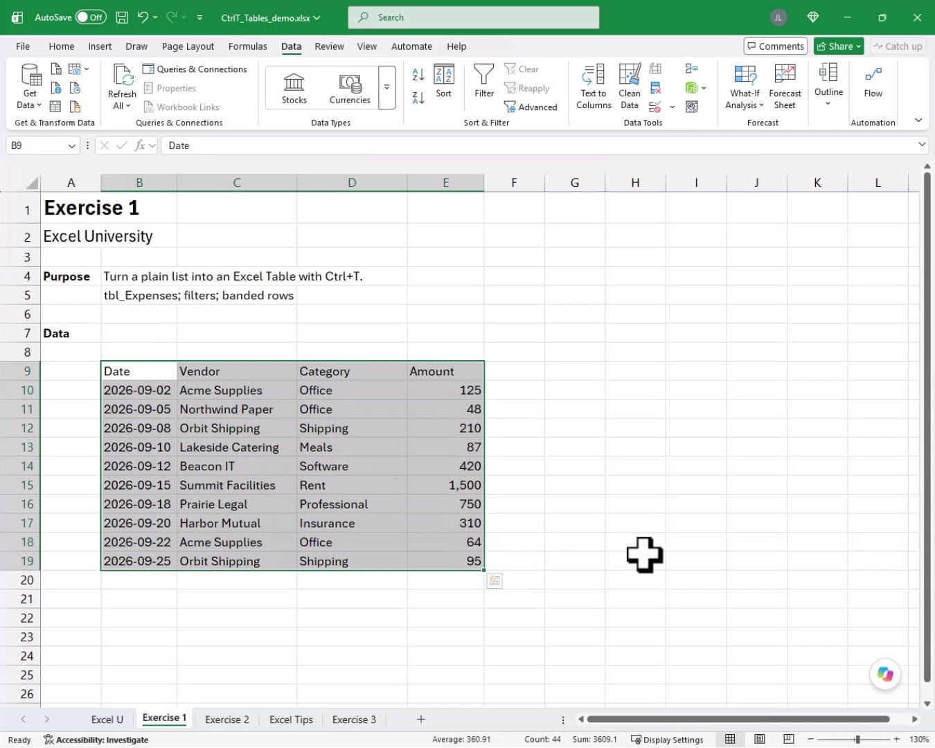
To convert it to a formal Excel Table, we click anywhere inside the range and press Ctrl+T. The Create Table dialog appears and confirms the range automatically. We also get a chance to give the table a name. Rather than leaving the default generic name, we type something descriptive like tbl_Expenses and click OK.

We hit Enter, and bam:

The range transforms into a styled Table with banded rows and filter dropdowns on every header. A new contextual ribbon tab, Table Design, appears whenever we are working inside the Table. From there we can toggle the Header Row, Total Row, Banded Rows, First and Last Column formatting, Banded Columns, and Filter Buttons on or off. We can also choose from a gallery of table styles.
The built-in filter buttons are immediately useful. We can click the Category dropdown, choose specific categories, and filter the view in seconds. When we are done, we clear the filter and all rows return. And that is how we can turn a plain range into a powerful Ctrl+T Table. Mission accomplished!
Exercise 2: Auto-Expanding Formulas and the Total Row
Now that we understand what a Ctrl+T Table is, it is time to see the feature that matters most for everyday work: auto-expansion. Let’s look at what happens with an ordinary range first, so the contrast is clear.
The Problem with Plain Range References
Consider the following worksheet, where we have the same expense data stored as a plain range. We want to sum the Amount column, so we write a formula in cell C8:
Before we write the formula, a quick look at the SUM function. It returns the total of all values in a range or list of values. The function arguments are:
- number1: the first number, cell reference, or range to add
- number2, …: additional numbers, references, or ranges to add (optional)
=SUM(E13:E22)

This works great right now. But the instant we add a new row below row 22, that row falls outside the formula’s range. The SUM does not update.

The total stays at 3,609 even though we added 100 in row 23. The formula is locked to E13:E22, and it has no idea a new row exists. This is the classic plain-range trap.
The Table Solution: Structured References
Let’s try the same thing with a Ctrl+T Table. After pressing Ctrl+T and naming the table tbl_exp, we write the SUM formula again. This time, when we click to select the Amount column data inside the Table, Excel automatically switches to a structured reference:
=SUM(tbl_exp[Amount])

A structured reference uses the table name followed by the column name in square brackets. It always refers to every data row in that column, no matter how many rows there are. Now we add a new row with a value of 100, and bam:

The total updates to 3,709 the instant we press Enter. The Table expanded automatically to include the new row, AND the structured reference formula picked it up without any manual adjustment. This is a very simple way to future-proof our workbooks.
The Built-In Total Row
If a grand total at the bottom of the Table is all we need, there is an even faster option. We click any cell inside the Table, go to Table Design, and check the Total Row checkbox. Excel adds a Total row directly to the bottom of the Table.

One common concern is that the Total row might block new data entry. Not a problem. When we reach the last cell in the last data row and press Tab, Excel loops to the first column and automatically pushes the Total row down. We can also paste new rows by selecting the Total row label and pasting, and Excel pushes it down the same way. The Total row always stays at the bottom.
Exercise 3: PivotTables Built on a Ctrl+T Table
Now, it is time to make things more interesting. The auto-expansion benefit does not stop at formulas. PivotTables built on a Ctrl+T Table also pick up new rows, so refreshing the PivotTable is all it takes to see updated results.
We convert our data to a Table named tbl_pt, then go to Insert, PivotTable. Excel uses the table name as the data source automatically. We place the PivotTable on the existing worksheet, drag Category to Rows and Amount to Values, and the PivotTable correctly summarizes our data. We also turn on the Total Row to confirm both match at 3,609.

Now we add a new row to the Table with a value of 100. Because the Table auto-expanded, the PivotTable only needs a refresh to include the new data. After refreshing, the Grand Total updates to 3,709, matching the Table’s Total row exactly.

No need to redefine the PivotTable’s source range. No need to update any formulas. The Table does the heavy lifting for us. And that is how we can use Ctrl+T Tables to keep PivotTables automatically in sync. Mission accomplished!
Summary
Ctrl+T Tables are one of those Excel features that deliver outsized value for minimal effort. We convert a plain range to a Table with a single keystroke, give it a descriptive name, and instantly gain banded rows, filter buttons, structured references, an optional Total Row, and auto-expansion. Formulas using structured references like =SUM(tbl_exp[Amount]) automatically include new rows as they are added. PivotTables built on a Table source stay current with a simple refresh. So those are a few different ways that Ctrl+T Tables can help us build more reliable, maintainable workbooks.
If you have any suggestions, improvements, alternatives, or questions, please share by posting a comment below … thanks!
Sample File
FAQs
What is a Ctrl+T Table in Excel?
A Ctrl+T Table, also called an Excel Table or table object, is a structured range that Excel treats as a named, dynamic data container. Unlike a plain range, it auto-expands when we add new rows or columns, supports structured references in formulas, and unlocks special features like the Total Row and Table Design ribbon tab.
How do we create an Excel Table?
We click any cell inside our data range and press Ctrl+T. The Create Table dialog asks us to confirm the range and enter a table name. We give it a descriptive name, check that the My table has headers box is checked, and click OK. Alternatively, we can go to Insert, Table from the ribbon.
What is a structured reference?
A structured reference is the way Excel references data inside a Table. Instead of a cell address like E13:E22, it uses the table name and column name in square brackets, such as tbl_exp[Amount]. This reference always points to all data rows in that column, regardless of how many rows exist.
Why does a SUM formula miss new rows in a plain range?
When we write =SUM(E13:E22), Excel locks the formula to exactly those rows. If we add a row in E23, it falls outside the formula’s range and is ignored. A structured reference like =SUM(tbl_exp[Amount]) avoids this problem entirely because it refers to the whole column inside the Table, which grows automatically.
What is the Total Row and how do we turn it on?
The Total Row is a built-in summary row that appears at the bottom of an Excel Table. We turn it on by clicking any cell inside the Table, going to the Table Design ribbon tab, and checking the Total Row checkbox. By default it shows a sum for numeric columns, but we can click the dropdown in any Total Row cell to choose a different function like Average, Count, or Max.
Does the Total Row block adding new data?
No. When we reach the last data cell in the Table and press Tab, Excel moves to the first column of a new row and automatically pushes the Total Row down. We can also paste new rows by selecting the Total Row label cell and pasting, and Excel shifts the Total Row down to accommodate the new data.
How do we give a Table a descriptive name?
We can set the name during the Create Table dialog when we first press Ctrl+T, or we can rename it afterward by clicking inside the Table, going to the Table Design tab, and editing the Table Name field in the upper-left corner of the ribbon. A good naming convention is a prefix like tbl_ followed by a descriptive word, such as tbl_Expenses.
Do PivotTables built on a Ctrl+T Table automatically include new rows?
Yes, with one small step. Because the PivotTable’s data source is the Table name rather than a static range, it knows where to look. When we add new rows to the Table and then refresh the PivotTable (right-click, Refresh), it picks up the new data automatically. No source range update is needed.
Can we convert a Table back to a plain range?
Yes. We click inside the Table, go to Table Design, and click Convert to Range. Excel asks us to confirm, and when we say yes, the Table formatting may remain but the data is converted back to a plain range. Structured references in formulas will also revert to standard cell references.
What versions of Excel support Ctrl+T Tables?
Ctrl+T Tables have been available since Excel 2007, so virtually all modern versions support them, including Excel 2010, 2013, 2016, 2019, 2021, and Microsoft 365. The core auto-expansion behavior and structured references work the same across all of these versions.

Excel is not what it used to be.
You need the Excel Proficiency Roadmap now. Includes 6 steps for a successful journey, 3 things to avoid, and weekly Excel tips.
Want to learn Excel?
Our training programs start at $29 and will help you learn Excel quickly.