Create a Dynamic PivotTable Style Report with One Formula

Historically, we’ve had two basic ways to create reports in Excel. We could enter the report labels and use formulas to compute the report values or we could use a PivotTable. Both options had pros and cons. We’d have to pick the report type based on the context of our workbook. In this post, I’ll show you a new option that use a dynamic array (DA). Specifically, we’ll write a DA formula with the new VSTACK and HSTACK functions to create a dynamic PivotTable-style report that automatically updates values and expands to include new items. No manual Refresh needed!

Formula-based vs PivotTable Overview

Before we jump in, let’s just back up a sec and recap the key pros and cons of traditional formula-based reports and PivotTables. We need to understand these details in order to fully appreciate the beauty of the new solution that VSTACK/HSTACK enables.

Formula-based reports

One approach to building reports is to enter the report labels into cells, and then write formulas that compute the report values. Since the report values are computed with formulas, they automatically recalculate anytime the dependent cell values changed. But, the problem is that they do not automatically expand to include any new items found in the updated data source. Meaning, if there is a new report label needed (found in the underlying data), you would need to manually insert a new worksheet row into your report, enter the new label, and then write or fill the formula to compute the value. The inability to auto-expand to include new items (new report label rows) has been a major bummer. This is why PivotTables have been such an amazing alternative to formula-based reports.

PivotTable Reports

PivotTable reports do automatically adjust their size to accommodate any new items found. That is, a PivotTable will automatically insert new report rows for any new items found in the underlying data. That is awesome and one of the many reasons Excel users adore PivotTables. The only little problem is that users need to remember to manually click Refresh after changing the source data in the workbook.

Options

And, these have been our two basic options for literally decades. We would need to make a choice between these two options based on our workbook. On the one hand, we could create a formula-based report that recalcs the values hands-free … but … we would need to manually insert new report rows and fill formulas. On the other hand, we could create a PivotTable that automatically includes new items … but … we would manually Refresh.

For years, I’ve wished for the best of both worlds. A formula-based report that would automatically recalculate values and dynamically expand to include new report labels (items).

Well, friends, this wish has finally come true!

With the introduction of VSTACK and HSTACK, we are able to build such a report. Probably, the most beautiful report of all. And, I’ll walk through all of the details in this post. Let’s go.

Disclaimer: I am not suggesting that we stop using PivotTables, or that DA functions can replace all PivotTables. For the record, I love PivotTables. I’m also not saying that there are no cons to the approach presented. I am saying that it avoids two of the cons noted above, mainly, formula reports don’t include new items and you need to manually Refresh a PT after you change table values. However, I wanted to talk about VSTACK/HSTACK with this set up so that we can see one really cool way to apply them. It is just another option that can help in some of our reports 🙂

Objective

Here is a screenshot of a traditional formula-based report.

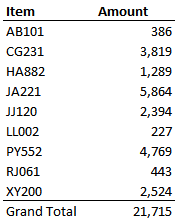
To create it, I manually entered the report labels and then used the SUMIFS function to create the values. The pro is that any new transactions in my data table are automatically included in the report provided their label is found in the report. The con is that when there is a new item, such as ZZ400, we need to insert a new worksheet row, type the new label, and then write or fill the formula to compute its value.

On the other hand, here is the PivotTable version of that report:

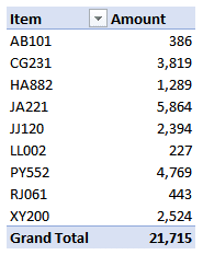
To create it, I used Insert > PivotTable, and added the items fields to rows and the amount field to values. The pro is that all new transactions are reflected in this report when I refresh it, even if a new report label (row item) is found. The con is that I need to remember to manually Refresh the report. This doesn’t take long, but, it is a step I need to remember to do, and if I forget the report will be inaccurate.

Now, here is a DA report that combines these two pros without inheriting the two cons.

It will automatically include new row labels like a PivotTable, and update its values all hands-free (no manual refresh) like a formula-based report. In fact, it is a formula-based report, but it uses Dynamic Arrays and the VSTACK/HSTACK functions.

Video

Narrative

Ready to get started? There are a few functions we‘ll be using:

1. HSTACK
2. VSTACK
3. LET

We’ll make these work together to create our Beautiful report. Let’s do it!

Note: not all versions of Excel include these functions. The fastest way to determine if your version of Excel supports them is to type =VS into any blank cell. If VSTACK appears in the auto-complete list then you have them! It is currently available only through an Office 365 subscription, and enhancements are pushed out based on your update channel (with the Insiders channel receiving updates first). You can control the update channel by going to File > Account > Update Options. If you are on a corporate network, your IT team may be able to assist.

HSTACK

The purpose of HSTACK is to combine columns of data side by side. In the case of our Beautiful report, we’ll first be using it to create the three main components of our report. We’ll think about writing individual formulas to create the header row, the body, and the total row.

Starting with the header row, we combine the report labels ItemNum and Amount like this:

=HSTACK("ItemNum", "Amount") 

Moving into the body of the report, we populate the report label column using the SORT and UNIQUE functions. These will sort the unique values found in the ItemNum column of our data table.

=SORT(UNIQUE(tbl_data[ItemNum]))

The second column in the body will populate the values for our Amount column. To do that, we’ll use the SUMIFS function to add up the amounts in the Amt column.

=SUMIFS(tbl_data[Amt],tbl_data[ItemNum],E8#) 

Next, we create the Grand Total row using the HSTACK function again. 

=HSTACK("Grand Total",SUM(tbl_data(Amt)))

The result of these four individual formulas will get us close to our desired report:

We are close, but we need to find a way to stack them together. Otherwise, our tables won’t auto-expand because our existing formulas will be in the way. 

That’s when we move on to our second function, VSTACK.

VSTACK

While HSTACK combines columns of data side by side, VSTACK combines tables vertically. We’ll use it to stack our row headers (E7#), the bodies of both report columns (E8#,F8#), and then our total row (E18#).

=VSTACK(E7#,HSTACK(E8#,F8#),E18#)

You can see how the formula arguments correspond to the previously computed ranges here:

Now that we have figured out our overall approach (compute the separate report regions and then VSTACK/HSTACK them together), we want to eliminate the helper references and write a single formula that will stand on its own.

One option is to replace the spill references in our formula (E7#, E18#, and so on) with the underlying function. That is, we can copy the individual formulas from the helper cells and paste them into our new VSTACK formula. This is the final result:

=VSTACK(HSTACK("ItemNum","Amount"),HSTACK(SORT(UNIQUE(tbl_data[ItemNum])),SUMIFS(tbl_data[Amt],tbl_data[ItemNum]),SORT(UNIQUE(tbl_data[ItemNum])),HSTACK("Grand Total",SUM(tbl_data[Amt]))

Now that our formula no longer needs the helper references, we can delete the temporary report we made and bam:

However, as you can see, we’re still left with one pretty long (and hard-to-maintain) formula. 

We can use LET to wrap it all up in one container and keep things organized (and easier to update and maintain over time). 

Putting it together with LET

The LET function allows us to assign names and then reference the names in the final calculation argument. In our case, we can assign the letter “r” to the expression that returns our row labels, “v” to the expression that computes our report values, “headers” to the function that creates the report headers, “body” to the HSTACK(r,v) function that provides our report body, and footer to the function that returns the total row. The final argument uses the VSTACK function to combine the headers, body, and footer. The full formula looks like this:

=LET(r,sort(UNIQUE(tbl_data[ItemNum])),
v,SUMIFS(tbl_data[Amt],tbl_data[ItemNum],r),
headers,HSTACK("ItemNum","Amount”),
body,HSTACK(r,v),
footer,HSTACK("Grand Total",SUM(tbl_data[Amt])),
VSTACK(headers,body,footer))

We hit enter, and bam:

Conditional Formatting

The last step in creating our Beautiful report is using conditional formatting to create a border between the values in the body of our table and the Grand Total section.

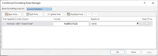
In this case, we’ll set a rule that says: apply a top cell border if the value in column B is equal to the word “Grand Total.” This will allow the cell border to change dynamically along with the cell values as we update the report.

Conclusion

With HSTACK and VSTACK, we’ve been able to work around the two identified cons of traditional formula-based reports and PivotTables. We now have the best of both worlds – a hands-free Beautiful report that automatically recalculates values and dynamically expands to include new items. No more extra steps or having to click refresh!

This is a pretty cool application of dynamic arrays, and it helps to overcome two key issues with traditional reports. Let me know what you think about it by posting a comment below…Thanks!

Sample File