Conditional Averages with AVERAGEIFS

The AVERAGEIFS function can compute averages for transactions that meet a set of criteria. In this post, we’ll use it to create a report by customer that ignores zero value transactions.

Overview

Although SUMIFS was probably the most popular multiple condition function introduced in Excel 2007, it wasn’t the only one. Microsoft released AVERAGEIFS which also supports multiple conditions. What are multiple condition averages? They are averages based on a column of numbers that include rows that meet one or more criteria. For example, we can compute the average of the amount column, but only include those rows where the customer column is equal to our customer and where the amount is not equal to zero.

Details

The AVERAGEIFS function arguments begin with the column of numbers to average, such as an amount or quantity column. The remaining arguments come in pairs, first the criteria range and then the criteria value. Up to 127 criteria pairs are supported. The function syntax follows:

=AVERAGEIFS(average_range, criteria_range1, criteria1, ...)

Where:

• average_range is the column of numbers to average
• criteria_range1 is the first criteria range
• criteria1 is the first criteria value
• … remaining criteria range/value pairs

The criteria value arguments can be expressed in many ways, including text strings such as “<>0” or cell references, and support wildcards.

Example

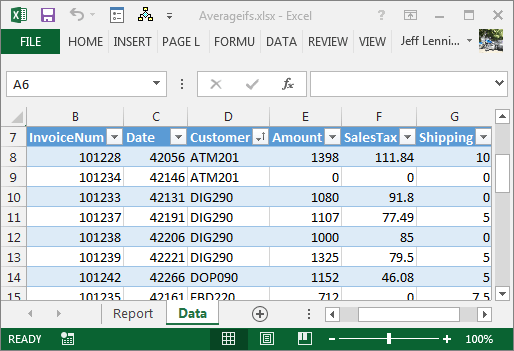
Let’s use an example. We’ve exported some transactions from our accounting system, and have stored in them in a table named Table1, as shown below:

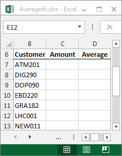
We would like to build a summary report by customer to display the sum and average for each customer, as illustrated below:

We can easily bust out the SUMIFS function to populate the amount column. Since we previously explored the details of the SUMIFS function, we’ll skip the mechanics of it and focus on the AVERAGEIFS function.

The idea is to average the table’s amount column, but only include those rows where the table’s customer column is equal to our customer. For example, the formula we would write in D7 above is:

=AVERAGEIFS(Table1[Amount],Table1[Customer],B7)

Where:

• Table1[Amount] is the column of numbers to average, the table’s amount column
• Table1[Customer] is the first criteria range, the table’s customer column
• B7 is the first criteria value, our customer

The results are displayed below.

And we are done…right? We’ll, it depends. It depends on if we want the average include or exclude zero values. If you’ll notice in the first screenshot, customer ATM201 has two transactions, one of which has a zero value. The current report includes the zero transaction in the average. If we want to ignore the zero transaction when we compute the average, we can simply add one additional criteria pair, as follows:

=AVERAGEIFS(Table1[Amount],Table1[Customer],B7,Table1[Amount],"<>0")

Where:

• Table1[Amount] is the column of numbers to average, the table’s amount column
• Table1[Customer] is the first criteria range, the table’s customer column
• B7 is the first criteria value, our customer
• Table1[Amount] is the second criteria range, the table’s amount column
• “<>0” is the second criteria value, does not equal zero enclosed in quotes

When we update the formula, the report ignores the zero value transaction, as illustrated below:

If you have any other preferred approaches, please post a comment below!

 Additional Resources

• Download sample file: Averageifs
• Posts about SUMIFS: Topic SUMIFS