VLOOKUP Hack #6: Different Data Types

We started this blog series by examining the 4th argument. We’ve since hacked the 3rd argument and then the 2nd argument. Now, as you can imagine, it is time to hack the 1st argument. There are many fun hacks we can do with the 1st argument, so, I’ll cover them over a few posts. In this post, we’ll address the data type issue.

I’ve prepared a short video as well as a full narrative below for reference.

Video

Objective

Before we dig into the details, let’s understand the issue. The issue is that with VLOOKUP, equivalent values stored as different data types don’t match. Let’s unpack this statement.

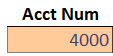
It is important to know that cells can store different kinds of values, such as numbers, text strings, dates, and Boolean values. When we type 4000 into a cell, Excel typically recognizes this as a number and stores it as a number. By default, Excel right-aligns numbers as shown below.

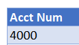
But, sometimes, especially when we import data from other sources, Excel can make assumptions about the data type and actually store 4000 as a text string. By default, Excel left-aligns text strings as shown below.

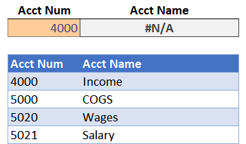
If we use VLOOKUP to match these two values (one stored as a number and the other as a text string), it will not make a match. This is because 4000 is stored as a number in one place and a text string in another place. In summary, VLOOKUP won’t match equivalent values when stored as different data types. When we try to retrieve the Acct Name based on the Acct Num, we get an error, as shown below.

So, apparently, we need to convert data types manually in order to use VLOOKUP. Or…do we? That brings us to the hack.

Hack

Rather than convert the data types manually, we have the option to handle the data type issue within the VLOOKUP function. We just need an assist from another function, the TEXT function.

Hack #6: Use TEXT as the 1st VLOOKUP argument

The TEXT function converts a number into a text string. By using TEXT as the first argument, VLOOKUP will make the match.

There are two arguments to the TEXT function, the first is the value to convert, and the second is the format code. Since we aren’t returning results to a cell, we don’t care about the format code and can just use 0 as the second argument. For example, if a number was stored in A1 that we wanted to convert to a text string, we’d use this:

=TEXT(A1,0)

When using it as the first VLOOKUP argument, it would look something like this:

=VLOOKUP(TEXT(A1,0),Table1,2,0)

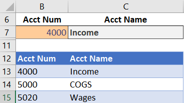
So, if we revisit our broken function, we can fix it with the following:

=VLOOKUP(TEXT(B7,0),Table1,2,0)

Yes…it worked, as shown in cell C7 below.

If we needed to do the opposite, and convert text values into numbers, we would use the VALUE function instead. It only has one argument, so, it looks something like this:

=VALUE(A1)

Or, if we used it as the first VLOOKUP argument, it would look like this:

=VLOOKUP(VALUE(A1),Table1,2,0)

Or, if we needed to write a function that worked for text and numbers, we could use our friend IFERROR, which we discussed in a previous post.

Essentially, the formula would try to match the number, and if it was an error, it would try to match the text string, like this:

=IFERROR(VLOOKUP(VALUE(A1),Table1,2,0),VLOOKUP(TEXT(A1,0),Table1,2,0))

That helps us cover our bases, and works when matching text-to-text, text-to-number, number-to-text, and number-to-number. Nice 🙂

But hang on Jeff, that feels like a lot more work than just converting the data types manually. And, if this were a one-time project, I would agree that it probably makes sense to manually convert the data types. But, on recurring-use workbooks, I prefer to eliminate such manual steps. So, using a formula like the one above in our recurring-use workbooks helps us work with the data as it comes.

The sample file below has these examples along with the formulas in case you’d like to take a look.

If you have any other fun VLOOKUP hacks, please share by posting a comment below, thanks!

• Sample File: Hack 6.xlsx