Split Amount into Monthly Columns

Let’s say you need to take an amount and split it evenly into monthly columns. For example, perhaps you need to recognize revenue over time. Or, perhaps you have spent some money and you need to allocate the expense over time. There are other illustrations, but the basic idea is that you have a total amount that you need to spread evenly into monthly columns. As this is Excel, there are many possible approaches. In this post, I’ll present a solution that uses dynamic arrays. The benefit of this solution is that you can quickly and easily adjust the number of columns displayed in the report. I’ve prepared a video and full narrative below.

Video

Objective

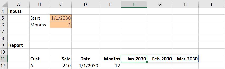
To illustrate this idea, let’s say we collect money up front for subscriptions we sell. For example, a customer may pay us $240 for an annual subscription. We basically need to recognize this revenue over time as it is earned. Since $240/12 months = $20, we would like our worksheet to show twelve monthly columns with $20 each. The first few months are shown below:

Our worksheet needs to include one row for each subscription sold to our customers. Each subscription could have a different start date, term, and amount. Perhaps something like this:

Our goal is to write one formula and fill it down, and we want it to work for all subscriptions. Plus, we want to be able to change the columns displayed in the report at any time, including the start date and number of months. And when we do, we want all of the formulas to update accordingly.

To tackle this, we’ll leverage dynamic arrays and the SEQUENCE and EOMONTH functions.

Details

We’ll compute our worksheet using the following steps:

• Dynamic month labels
• Monthly true/false
• Monthly amount

Let’s get to it.

Note: this solution uses dynamic arrays and the SEQUENCE function. Depending on when you read this post, your version of Excel may or may not support these. As of the time of this writing, these features are available only in the O365 version of Excel. If you have a version of Excel that doesn’t support dynamic arrays or the SEQUENCE function, check out this previous post instead. 

Dynamic Month Labels

First up, let’s tackle the monthly column labels. We want these to be dynamically generated based on the Start date and Months entered by the user. We will provide two input cells, like this:

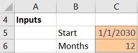
Based on the values entered, we want Excel to automatically create the monthly column labels.

To accomplish this, we need to understand how two functions work: EOMONTH and SEQUENCE. Let’s take them one at a time, and then combine them.

EOMONTH

EOMONTH computes the last day of the month, given a start date and the number of months to offset. For example:

=EOMONTH(start_date, months)

So, if start_date is 1/1/2030, and months is 0, then EOMONTH returns 1/31/2030. If start date is 1/1/2030 and months is 1, then EOMONTH returns 2/28/2030, and so on.

SEQUENCE

SEQUENCE returns a numerical sequence, given a start value.

=SEQUENCE(rows, [columns], [start], [step])

We can specify the number of rows and columns we would like returned, as well as define the starting value. For example, we could request 12 rows starting at 1 to return an array of values 1 through 12. The step value tells Excel the increment value, and defaults to 1 if omitted.

EOMONTH/SEQUENCE

Now, let’s put these two functions together. If we want Excel to automatically generate the requested number of monthly columns (C6 in screenshot above), starting with the month entered by the user (C5 in screenshot above), we use SEQUENCE as the months argument of EOMONTH, like this:

=EOMONTH(C5,SEQUENCE(1,C6,0))

As the user enters various values for start date and number of months, the column labels update accordingly.

So cool!

Note: you’ll want to select the entire row (11) and apply the desired date format. In the screenshot above, I used the custom date format mmm-yyyy. But, you can pick any date format desired. 

Monthly TRUE/FALSE

With the monthly column labels working, we need to identify which columns should get the monthly amounts, based on the subscription start date, computed end date, and monthly column labels.

Basically, if the monthly column label falls between the subscription start date and the computed subscription end date, then we should insert the monthly amount (subscription total divided by subscription months). However, if the column header is before the start date or after the subscription end date, then the column gets 0.

To identify which monthly columns should get monthly amounts, we will use Boolean true/false logic.

For starters, let’s determine if the subscription start date (D12) is less than the column label (F11). We can use a basic less than or equal to comparison operator, like this:

=D12<=F11

If we wrote the formula this way, it wouldn’t dynamically expand right along with the column headers. So, we need to use the spill range operator #, like this:

=D12<=F11#

Now, the formula returns multiple results, and those results spill right along with the column labels. We need one more adjustment to ensure that when we fill the formula down it will continue to work, so we update F11 to an absolute reference, like this:

=D12<=$F$11#

Now we need to address the subscription end date. Our goal is to see if the column label is less than the subscription end date. We can use EOMONTH to figure out the subscription end date. So, we can use the following expression to compare the column label with the computed subscription end date like this:

$F$11#<=EOMONTH(D12, E12-1)

To add this expression to our original formula, we need to use the multiplication operator for AND logic (both expressions need to be true for the column to get the monthly amount). So, our updated formula looks like this:

=(D12<=$F$11#)*($F$11#<=EOMONTH(D12,E12-1))

This formula returns 1 into the cells that need the monthly amount and 0 into the cells that don’t. We can fill the formula down for all subscriptions, and the results look like this:

All that remains is to compute the monthly amount for each subscription.

Monthly Amount

The basic expression to compute the monthly amount is the total sale divided by the number of months in the subscription. For example, for Customer A it would look like this:

=C12/E12

Since we already have 1s and 0s in the correct columns, all we need to do is multiply those results by the monthly amount. So, we update our formula like this:

=(D12<=$F$11#)*($F$11#<=EOMONTH(D12,E12-1))*(C12/E12)

When we fill the updated version down, we confirm the results look good:

And what I love about this solution is how dynamic it is. We can change the Start date or Months input values, and the report column labels and amounts update immediately.

If you have any other cool dynamic array or SEQUENCE tips, please share by posting a comment below … thanks!

Sample file: RevRecDA.xlsx

Note: if you download the sample file but your version of Excel doesn’t support dynamic arrays or the SEQUENCE function then you may receive formula errors and the columns won’t dynamically update as described in the article above.