Multi-Column Lookup with VLOOKUP and SUMIFS
When you need to perform a lookup, your instinct tells you to use VLOOKUP. But, when your lookup uses multiple conditions and columns, you may be inclined to use SUMIFS. However, when the value you need to return is a text string, rather than a numeric value, you are precluded from using SUMIFS since it only returns numbers. But, are you? This post demonstrates how to perform a lookup on multiple columns and return a text string by combining these two powerful functions. Excited? Me too! Let’s get to it.
Objective
Before digging into the mechanics, let’s be clear about what we are trying to accomplish.
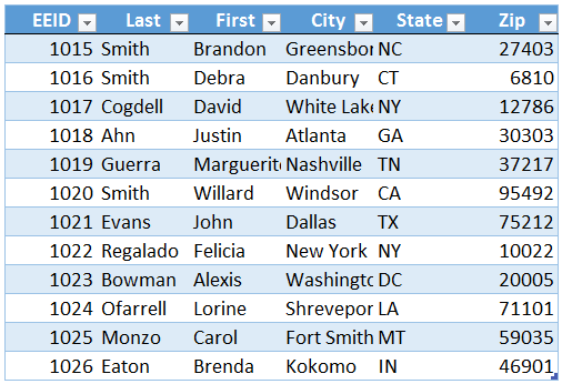
We have a bunch of employees stored in a table named Table1, as shown below.

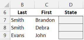
We are trying to build a report that retrieves the State given the employee Last and First names, as shown below.
If the report had contained the Employee ID instead of the Last and First name, the lookup would be easy, right? We could just use VLOOKUP and be done. But, our lookup needs to be performed by matching two columns, the Last and First name columns. If the value we were returning was numeric, such as the Zip code, we could use SUMIFS. But, since SUMIFS returns numbers and not text strings (such as the State), we can’t use SUMIFS. And since the lookup must be performed on multiple columns, we can’t use VLOOKUP. If we can’t use SUMIFS or VLOOKUP, then, what are we supposed to do? Well, what if we used SUMIFS and VLOOKUP in the same formula? Can we do that? Yep. Here’s how.
Details
We essentially use SUMIFS to return the unique Employee ID value, and then we feed that value into VLOOKUP as the first argument. This means that VLOOKUP has a lookup value that is determined by the SUMIFS function. SUMIFS will retrieve the EEID for the desired employee based on the Last and First name columns, and then VLOOKUP will use that ID to perform a standard lookup and return the State. In summary, we use the SUMIFS as the first argument of the VLOOKUP. Let’s take the functions one at a time.
Here is the report.
The data is stored in Table1. Let’s take the first step with the SUMIFS function. We want it to return the unique EEID. So, we use the following formula.
=SUMIFS(Table1[EEID],Table1[Last],B7,Table1[First],C7)
Where:
- Table1[EEID] is the column of numbers to sum
- Table1[Last] is the first criteria range, the last name column
- B7 is the first criteria value, the report’s last name value
- Table1[First] is the second criteria range, the first name column
- C7 is the second criteria value, the report’s first name value
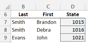
The results of filling this formula down are shown below.
We were able to use SUMIFS to retrieve the Employee ID based on matching the First and Last name values. So far so good? Now, we just need to ask VLOOKUP to return the State based on the Employee ID.
Note: it is important to note that this technique assumes that each EEID value is unique within the column, and that only one row will satisfy all SUMIFS conditions. If these assumptions are not met, this technique may not work as expected. If your data table doesn’t have a unique ID column, you can always add a helper column that numbers the records 1, 2, 3, and so on.
Let’s use the SUMIFS function above in a VLOOKUP, as shown below.
=VLOOKUP(SUMIFS(Table1[EEID],Table1[Last],B7,Table1[First],C7),Table1,5,0)
Where:
- SUMIFS(…) returns the Employee ID for use as the VLOOKUP’s lookup value
- Table1 is the lookup range, the employee table
- 5 is the column that has the value to return, the State column
- 0 tells Excel we are looking for an exact matching EEID value
After filling the formula down, our report is complete, as shown below.
We did it…yay!
Note: It is also interesting to note that this technique can be used with date columns as well, and if needed, we could use comparison operators to find values within a range of dates.
If you have any other techniques for performing multi-column lookups, please share by posting a comment below…thanks!
Additional Resources
Excel is not what it used to be.
You need the Excel Proficiency Roadmap now. Includes 6 steps for a successful journey, 3 things to avoid, and weekly Excel tips.
Want to learn Excel?
Our training programs start at $29 and will help you learn Excel quickly.


Thanks! It is an interesting trick.
This is a great solution. It solved my problem 100% Thank you.
I have worded for the City of Wentzville for 24+ years and do payroll/software functions. I do manually an attendance history report for each employee (currently we have 200+ employees) on their days off while I balance their vacation, sick, comp, floating holiday and safety day balances by month. We currently purchased a new attendance system where I can download a .CSV file and import into Excel Spreadsheet. I came up with a huge spreadsheet listing everyday of the year for each employee times 3 lines (one for Vacation, one for Sick, and one for Comp). Got this all setup, where it will add and subtract to give me a balance for each benefit. Then I realize I would need to merge this into a Word Document and to do that you have to make all your numbers text, so no calculations. Could you please suggest a good way to do this. There is other information on this form, like vacation max for year, hourly wages, hire dates, pay grade, name, employee #, title, etc.
Any words of wisdom would be greatly appreciated. I have been thinking about this for years, it is sort of a do or bust project. LOL!! Thanks so much. If it would be easier I could scan a form to you so you could see what I am trying to accomplish. Mary Berscheid
Mary,
My best suggestion would be to get the Excel file to perform all of the computations, like you are doing, and be sure that your summary in Excel has one row per employee. Then, you can use the Microsoft Word mail merge feature. This will allow you to set up a standard letter, and retrieve the key values (merge fields) from the Excel file. There are several output options for the Word mail merge, including one great big Word file, PDF files, Emails, and more. Hope it helps!
Thanks
Jeff
VERY USEFUL .
THANKS
Hi- I need help on following table to combine vlookup and sumif.
Table :
A -2
A 4
A -3
B -4
A -4
B 7
I need formula to calculate only for negative sum from column 2 and vlookup for column.
Results should be like this
A -9
B -4
Can you help to create formula for this?
Thanks, Rahul
You can use SUMIFS to do that, just set one condition to the A or B value and the other condition to “<0" and you should be set.
Thanks
Jeff
Thanks Jeff. I am dealing with a different kind of issue though on similar lines which I hope you can guide me. I have multiple worksheets and a master sheet. Master needs to have data from individual worksheets. But the issue is that the text I want to lookup on master is existing on multiple worksheets at the same time and I would like the sum of all of it on master tab. So if I am looking up on name ‘John’ on master, the name John exists on 3 worksheets and I want a total of values against the name John on master. Any ideas on how to achieve this!
A macro can be used for this with a variable for the index number of the sheets.
I have a list of approximately 400 student’s names by class and number. On another sheet, I must make new seating charts every term.
Class, Number, Name
1, 1, Yamamoto Jun
1, 2, Fujiwara Ken
1, 3, Kusakabe Mei
…
2, 1, Honda Kuruma
2, 2, Yamamoto Ryo
2, 3, Kusakabe Satsuki
…
10, 1, Sakurai Ryo
10, 2, Hashimoto Kenta
10, 3, Yamamoto Non
…
On the seating chart sheets I want to enter a class number and student number and have the name appear below them.
I am revamping a system which uses VLOOKUP with the student number as the lookup_value, but this requires 11 sheets and a different table_array for each of them. Is there some way to have the table_array include all the students and be able to return the appropriate student name?
For example; if cell C11=2 and C12=3, I want D11=Kusakabe Satsuki
For lack of knowledge of a more elegant method (if one exists), I tried this:
1. Added a column at the left of the “List of names” sheet and concatenated the Class (one or two digits) and Number (padded to two digits)
=TEXT(B2,”##”)&TEXT(C2,”00″)
2. Put the Class on the Seating Chart sheets (L2) and modified the VLOOKUP
=IF(A7=””,””,VLOOKUP(TEXT($L$2,”##”)&TEXT(A7,”00″),’List of names’!$A$2:$H$350,4,FALSE))
*A7 is the cell where the Number would be entered for the first desk
When seating changes need to be made, I can just enter the Number at a desk and reprint.
Now the formulas can be changed once and copied to the 45 different seats if modification is needed, and the sheets for each class are actually identical because there is just one table_array instead of eleven, so the sheets can be copied if formatting or formula modification is needed (or just use one sheet and change the class number).
Each year the table_array will need to be adjusted once for the number of students and copied.
The actual page has two lookups for students names in Japanese and English, but the formula difference is only in the col_index_number.
One option is to nest VLOOKUP and SUMIFS, such that SUMIFS handles the multiple conditions and VLOOKUP returns the text string. I’ve written a post about this technique in case it will help https://www.excel-university.com/multi-column-lookup-with-vlookup-and-sumifs/
Thanks
Jeff
Thank you for the reply. The concept sounds great so I will certainly read up on the post you linked.
This is a phenomenally cool trick; however, I think your caveat cannot be emphasized enough:
(from above blog post)
Note: it is important to note that this technique assumes that each EEID value is unique within the column, and that only one row will satisfy all SUMIFS conditions. If these assumptions are not met, this technique may not work as expected.
I AM PREPARING ATTENDENCE SHEET OF EMPLOYEES FOR AN YEAR.MONTHLY SHEET OF EMPLOYEES HAVE ALREADY PREPARED BUT AS A SUMMARY I NEED YEARLY PRESENT ABSENT DAYS OF EMPLOYEES IN MASTERS SHEET.HOW TO SUM UP VALUES ACROSS MULTIPLE SHEETS AND RESULT SHOULD BE DISPLAYED IN A SINGLE MASTER SHEET ACCORDING TO THEIR RESPECTIVE ID NUMBER.KINDLY HELP ME THROUGH THIS.
The practical application of combining these two functions is pretty neat.
If the data contains no column with a unique value to =SUMIFS(), then there is the option to work on a helper column.
It is all about learning the many ways to get to Rome.
Thank you, Jeff.
Hey,
I’m comparing purchase orders between my company and my supplier. We compare the PO#, ETA, customer # and quantity between each. Sometimes the PO#’s are used multiple times when the orders are large and are shipped at different times. I wanted to use this trick to match the PO# and the ETA from our data to theirs to populate the remaining cells and then compare using an IF function to highlight any discrepancies. This doesn’t seem to be viable since the main criteria ( the PO# ) isn’t unique. Does anyone have any ideas ? I can explain further if needed.