Most Recent Transaction Date

I recently received a question about how to find the most recent transaction date of a list of items. There are a few fun ways to accomplish this, and so I thought I’d walk through three options. Thanks Darrell for your question!

Objective

The exact question from Darrell is:

“I have a data table of sales information that I would like to be able to pull the last or most current date that a list of items was sold. Is there a date function that will allow me to do this?”

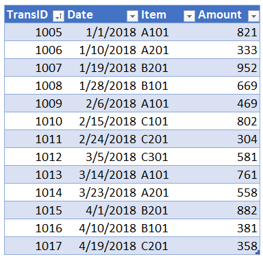
Based on this question, I imagine a table of sales transactions that may look something like this:

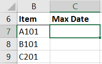
Then, we have a list of items for which we want to find the most recent sale date. It may look something like this:

As with just about anything in Excel, there are several ways to accomplish this task. And, we’ll look at three options and talk about when each may be a good fit depending on the purpose of the workbook. Sound like a plan? Great, let’s do this thing.

Options

We’ll look at the following three options:

• With a Formula
• With a PivotTable
• With a Get & Transform Query

We’ll take them one by one.

With a Formula

A formula-based option would be a good fit if you need to retrieve these values into specific cells in the workbook, for example, in a dashboard, KPI report, or other summary.

There are several functions we could use here, including traditional lookup functions such as VLOOKUP or INDEX/MATCH (which would work if the data was sorted descending by date), or MAXIFS if you have a modern version of Excel which supports it (thanks for the assist Donald!).

INDEX/MATCH

We’ll start with the INDEX/MATCH combination since these functions have been available for decades.

For this to work, we need to begin by sorting the transactions in descending order by date. That way, the first row encountered for each item will be the latest (most recent) transaction date.

The sorted table looks like this:

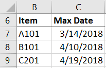
Now, our job is to simply retrieve the first date that appears for each of the selected items.

So, let’s say we enter the items in to some cells, like this:

Assuming our transaction table is named tbl_data, we would write the following formula into C7:

=INDEX(tbl_data[Date],MATCH(B7,tbl_data[Item],0))

The INDEX function returns a value from the tbl_data[Date] column, and the MATCH function tells the INDEX function which row. It returns the date from the first row where the item in B7 is found in the table’s item column tbl_data[Item]. The 0 argument value tells the MATCH function to use exact match logic.

We fill the formula down, and we have the max dates, as shown below.

MAXIFS

If your version of Excel has the MAXIFS function, this task will be much easier. We can simply use the following formula in C7:

=MAXIFS(tbl_data[Date],tbl_data[Item],B7)

And the best part is that the data does not need to be sorted!

So, a formula-based approach is one option. Let’s check out another option.

With a PivotTable

We can also accomplish this task with a PivotTable. This option would be a good fit if you perform this task frequently, and if the list of items is small. With a few items, it is really fast and easy to filter the PivotTable report for the desired items.

We start by selecting any cell in the data range, and then use the Insert > PivotTable command.

We insert the Item field into the Rows layout area, and then we insert the Date field into the Values area. At this point, the report looks something like this:

With the basic structure in place, we just need the cosmetics. First, let’s start by telling Excel to find the max date for each item. We do this by right-clicking any value in the PivotTable, and then selecting Summarize Values By > Max. The updated report is here:

Currently, the Max of Date column doesn’t look like a date because it is displaying the date serial instead of a formatted date. No worries, we can easily change the formatting. We right-click any of the date serials, and select Number Format (not Format Cells). In the resulting dialog, we pick our desired date format, and the updated report is looking good.

Now, we use the Row Labels drop-down to pick the list of items we want to see, and we remove the Grand Total by using the PivotTable Tools > Design > Grand Totals ribbon icon. The updated report is shown here:

We double-check the dates, and we confirm they are the same dates returned by the formula approach…nice!

Let’s head into our final option.

With a Get & Transform Query

A Get & Transform query (first built-in to Excel 2016 for Windows, formerly available as the Power Query add-in) would be a great fit for this task when there are tons of transactions and the list of selected items is long.

If you aren’t familiar with using Get & Transform queries, I’ll provide a link to additional G&T blog posts below for reference.

First, we select the items table and select the Data > From Table command.  (This command was first built-in to Excel 2016 for Windows). Since we don’t have any transformations, in the resulting Query Editor, we simply select Close & Load To.  Please note that Close & Load To is available by using the drop-down Close & Load button. In the resulting Load To dialog, we select Only Create Connection, as shown below.

Next, we do the same thing for the data table, and again, select the Only Create Connection dialog.

At this point, our workbook contains two query connections, one to the list of items and the other to the transactions. At this point, we just need to retrieve the max date from the data query for each item in the items query. To do this, we select

• Data > New Query > Combine Queries > Merge

In the resulting Merge dialog, we select the item query from the first drop down and then select the item column. In the second drop-down, we select the data query and again select the item column. By selecting the two item columns, we are telling Excel that these are the fields that have the matching item values. That is, they are the join field. Since we want the resulting query to show all items in the items query, and just the matching values from the data query, we accept the default Left Outer join as shown below.

The resulting query editor is shown below.

We expand the NewColumn table fields by clicking the icon in the NewColumn header, and selecting only the date column, as shown below.

We then select the Item column and click the Group By ribbon command. In the resulting Group By dialog, we create a new column name, such as MaxDate, select Max as the Operation, and select the Date column, as shown below.

Now, we just Close and Load to return the values to our workbook. After applying our desired date format, the results are shown below.

And look…they are the same values as the other two options. It worked…yay!

So, we examined three ways to accomplish the same task in Excel. Depending on the nature of your data and workbook, one option may be a better fit. Now, if you have an additional options, please share by posting a comment below…thanks!

Additional Resources

• Excel file: QA1.xlsx
• Additional Get & Transform blog posts: Get & Transform Posts
• Additional PivotTable blog posts: PivotTable Posts