Retrieve Values from Many Workbooks
Alright my friends, this week I’ll tackle a question I received about retrieving values from workbooks. Here is the basic idea of the question. I have a folder with several hundred workbooks, and each workbook may contain any number of worksheets. For example, some workbooks have two sheets, some have three sheets, and some have up to thirty worksheets. I need to create a single summary sheet that retrieves specific cell values from every sheet in all of these workbooks. Currently, I copy/paste, but, I want to automate this lookup process. Thanks Regina for your question, and for inspiring this post.
Objective
Let’s just be crystal clear about our objective. Here is the set up. We have a folder that contains hundreds of Excel files. And, just to make this a bit trickier, let’s assume that at any time, new workbooks can be added to the folder, or, some workbooks can be removed. In other words, our solution needs to adapt to a changing number of workbooks, and essentially grab values from all workbooks in the folder, however many there are at that moment.
Plus, workbooks do not contain the same number of worksheets. Some contain two, some three, and some up to thirty. Our solution needs to retrieve values from all sheets, plus, sheets may be added or removed at any time. And, there is no naming convention for the worksheets…they are named without any consistent pattern. So, our solution needs to adapt to this crazy and dynamic situation.
Plus, each worksheet may contain one or more values to retrieve. And, the values can appear on any row. So, it isn’t like we can use a formula that retrieves a value from say row 10…the value can appear on any row, and, there may be more than one value on each sheet. Craziness!
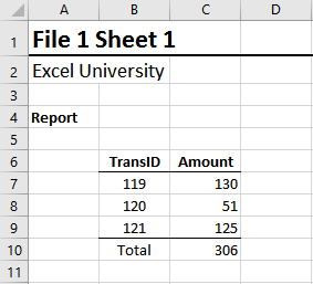
Now, we finally do get a bit of good news. The values we need are always stored in column C, and, Column B always contains the word Total next to the value. For example, here is the basic structure of each worksheet.
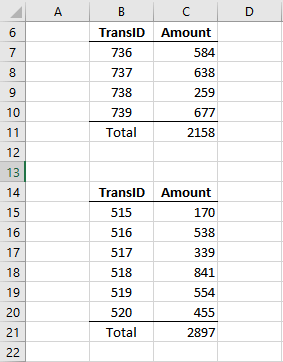
But remember, the total can appear on any row, and, some sheets have multiple totals, like this one.
So, our mission, should we choose to accept it, is to create a single summary sheet that retrieves values from various rows in any number of worksheets, in any number of workbooks in the folder. And, we want to be able to refresh our summary sheet at any time to capture the current values. Also, we don’t want to write any VBA code. And, going forward, we want to be able to update our summary in less than 10 seconds since we have to update it every day.
Can we do this? Yes, of course. We’ll explore how to accomplish all of this with a single Get & Transform query. Let’s get to it.
Details
We’ll accomplish our objective with three basic steps:
- Create a basic query
- Customize the query
- Return the results
This is going to be so fun!
Note: The steps below are presented with Excel for Windows 2016. If you are using a different version of Excel, please note that the features presented may not be available or you may need to download and install the Power Query Add-in.
Create a basic query
First we need to create a query that retrieves a list of all workbooks in the folder. This can be done by selecting the Data > New Query > From File > From Folder icon. Excel displays the Folder dialog (as shown below), and you can type or Browse to identify the folder that contains all of the Excel workbooks.
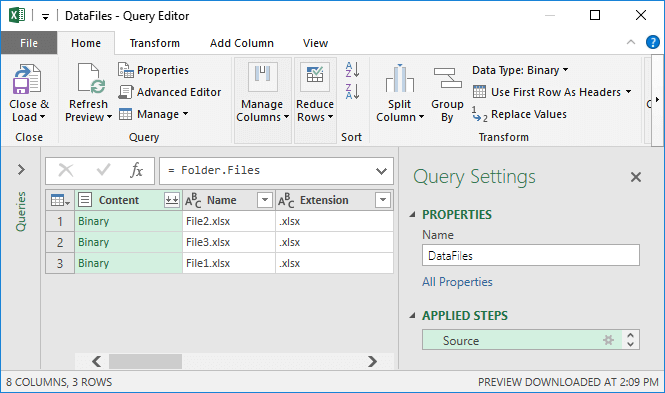
Clicking OK will display a preview dialog that lists the workbooks in the folder. Click the Edit button to open the Query Editor as shown below.
At this point, we have a query that retrieves the folder contents, and provides a list of all workbooks in the folder. With this basic query set up, it is time to customize it.
Note: if the folder contains a mix of file types, you can filter the Extension column to retain only the xlsx files.
Customize the query
At this point, we have a query that includes a list of the workbooks in the folder. Now we need to add a new column to include each worksheet in each of the workbooks. To do this from within the Query Editor, we select the Add Column > Add Custom Column command.
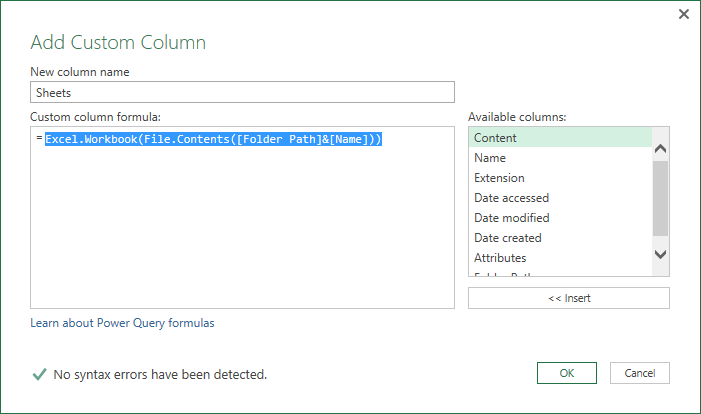
In the resulting dialog, we enter a name for our new column, something like Sheets would be fine, and then the formula:
=Excel.Workbook(File.Contents([Folder Path]&[Name]))
This is displayed below:
Click OK to add the new column to the query.
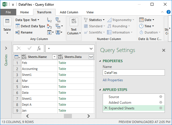
Our new column, Sheets, needs to be expanded. We can do this by clicking the little icon in the column header, or the Transform > Structured Column > Expand command. We can just expand all columns for now.
The query editor now includes all sheets and all workbooks, as shown below.
Note: if needed, apply filters to remove any rows that aren’t needed.
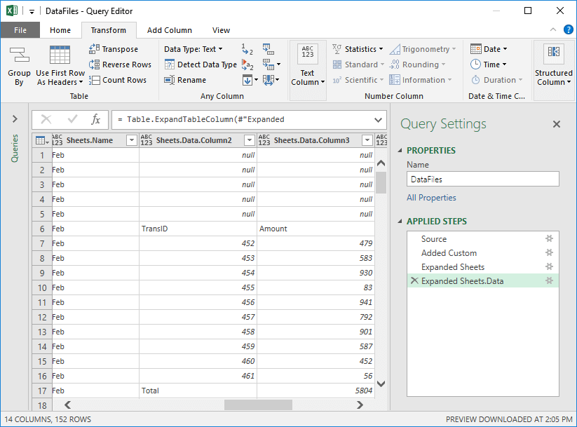
Next, we need to bring the sheet contents from columns B and C into the query. So, we expand the Sheets.Data column. We do this by clicking the little icon in the header, or by clicking the Transform > Structured Column > Expand icon. Since the Total label is in column B, and the Value in column C, we don’t need to bring in all columns, we can just check the Column2 and Column3 boxes.
Now our query includes the values from the worksheets, as shown below.
Now we have all the data we need! We just have to do some clean up and remove the rows and columns we don’t need.
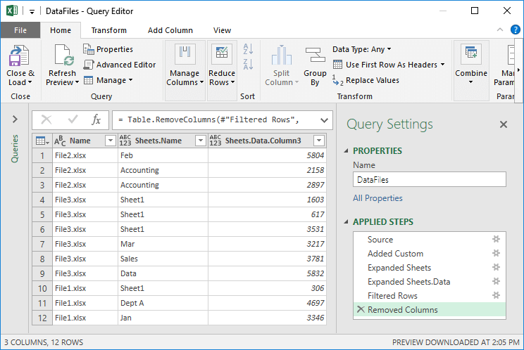
The only query rows we need to keep are those with the text string Total in Column2. So, we apply a filter by using the drop-down for Column2, and selecting Total. This leaves only the rows that include the total values we are seeking.
Next, we can remove any columns we don’t want or need returned to our summary sheet. We can pick and choose the columns and use the Remove Columns icon for this. Here, I’ve removed all columns except the ones that contain the workbook name, worksheet name, and value. The updated query is shown below.
Now, all the hard work is done! And we can just move on to the last step.
Note: thank you Ken Puls (Power Query guru) for your post.
Return the results
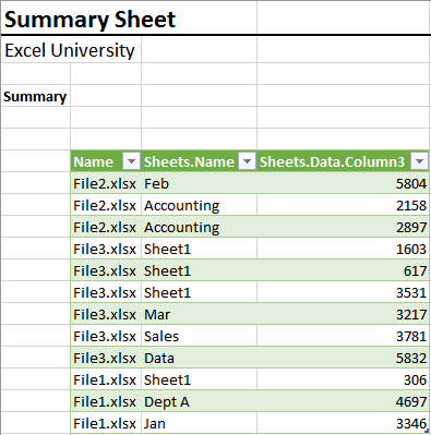
Finally, we can use the Close and Load command to return the query results to our summary sheet, as shown below.
Unbelievable…we did it! And, the best part is that we don’t need to go through all of that trouble next time we want to update the summary. We can simply right-click the results table and select Refresh. When we do, Excel goes back to the folder, and automatically includes any files that were added since last time. Plus, it automatically includes any new worksheets! And, it will retrieve the totals from all sheets, regardless of how many there are on each sheet or which row they are in. Wow!
But Jeff, come on man, we only had 3 files, I could have copy/pasted faster than that. Well, maybe, but, since this summary needs to be updated each day, week, or month, the Refresh will certainly be faster next period. Out of curiosity, I copied these three files, and pasted, pasted, pasted, and pasted, over an over, until I had about 420 Excel files in the folder. Then I hit Refresh. 6.76 seconds later, my summary table included 1,680 rows of data…freaking awesome!
If you have any other options to accomplish this task, or any other fun Get & Transform query tips, please share by posting a comment below…thanks!
Resources
- Sample data files (zipped): DataFiles
Excel is not what it used to be.
You need the Excel Proficiency Roadmap now. Includes 6 steps for a successful journey, 3 things to avoid, and weekly Excel tips.
Want to learn Excel?
Our training programs start at $29 and will help you learn Excel quickly.


Jeff, I had the same problem, but I worked it out somewhat in a different way. This example is used in a financial report for a year to date and a month report along with a previous YTD and month report all on one report. You pick/choose a report by picking from a drop down list indicating month and year. Once the timeframe is chosen all figures, calculations are updated to reflect that timeframe
At present my workbook is looking through 27 worksheets containing 6 columns and 229 rows of numbers of which 1 column is text.
In my program all worksheet reside in one workbook and each workbook has an ID name that reflects mth & yr. and each row has a individual account number that needs to be modified to reflect the month and year. This is done by running a VBA program which take seconds. Now one the master worksheet I have a number of hidden columns that will tie in the month and year from those worksheets by a vlookup formula and from that row where I want to return a number to reflect that year and month I use the following formula which is an array.
=VLOOKUP($E5,INDIRECT(“‘”&INDEX(SSheetList,MATCH(1,–(COUNTIF(INDIRECT(“‘”&SSheetList&”‘!$A$5:$G$232″),$E5)>0),0))&”‘!$A$5:$G$232”),3,FALSE)
I can add a new sheet and get results in less then 2 minutes and once added I can pick from my drop down mth. yr. list and have the worksheet updated in less than 10 sec.
Now this didn’t get made in a day or two, it took me a couple of days just to get this formula in place and working but now that I have it, it saves me 100’s of analyze hours.
That sounds awesome…I love hearing how Excel can help save time, and how there are typically multiple ways to accomplish any given task. Thanks for sharing your comment!
Can you do this if the files are in multiple folders? Can it bring back the name of the folder that it is in?
I ask because I’m collecting a large amount of A/P data that the main folder is information received, then it goes down to the vendor and from there has the file containing the ID number, address, etc. for that specific vendor.
Hi Mindy! Yes and yes! This same exact query will include all files AND subfolders in the source folder. The query includes a column for full path (folder) as well. Totally awesome!
Thanks
Jeff
Wow! that IS totally awesome! thank you!
Welcome 🙂
I use the Power Query, and love it. It is nice to be able to pull in information from other Workbooks, without changing the data, or missing some. We use it to combine several Sheets into one, for a month report, and then in another file, use Power Query to combine the months into the report for a YTD. We use 2013, and it does not have the Query option, so I learned the Power Query. Really nice and easy to use, once you understand it. I haven’t tried to have it figure the number of sheets per book, but that is something I will have to try. Thank you for another great post!
Power Query is a game changer…I love it too 🙂
Since I joined this site I have learned a lot and I love Excel it has really simplified my work. I also had interest in retrieval of data from various workbooks where we sell flowers to different clients with different varieties different invoices have to be raised and then reconcile at the end of the month giving different reports to the different departments, I have been trying to the formulae =Excel.Workbook(File.Contents([Folder Path]&[Name])) but on hitting enter it reports file contents cannot be found what could be doing wrong am on excel 2016.
Regards,
Geoffrey
Groove Ltd Naivasha Kenya
Thanks Jeff! Your explanation is excellent and Power Query is avesome. . I have troubled with the Query formulas several times! They seems to be case sensitive!
Ah, yes, they are case sensitive! A great book for learning more is M is for (Data) Monkey.
Thanks
Jeff
Thank you Jeff.
Your explanations and demos are very helpful.
Moshe
I have a question about this. I’m not sure if this is even possible or if this is even the best way to do what I want to accomplish. However, what I am trying to accomplish is this:
– I have a file full of employee attendance records. In the attendance records I put for example “A” for absence, “AA” for approved absence, “SI” for shift interruption, etc.
– On a completely different sheet, I want all those individual attendance records to communicate to this other “Time Off Request” sheet so if in “Bob’s” attendance record he has an approved absence (“AA”) that it will pop up on the right date in my “Time Off Request” sheet.
So the value the time off request sheet will be looking for is always “AA” but it could be on any given day, and from all the attendance records in the file. This way I can look at one day and see how many people are scheduled to be out that day.
So is this possible and is it doable with using this Power Query function or is there a different thing I could do to achieve this? I’m not super knowledgeable with excel, but I am also not completely terrible with it. Haha. Any help would work. Thanks!
Hi Sadie,
I think you are trying to find the count of the number of people with a given code, A, AA, or SI. I believe the COUNTIFS function may be able to help, as it provides the count of the number of rows where multiple conditions are true. For example, where the number of codes is AA. It can also count based on date conditions as well.
I’ve written an article about COUNTIFS here:
https://www.excel-university.com/articles/cal-cpa/comparing-spreadsheet-lists-with-ease/
Hope it helps you get started!
Thanks
Jeff
Thank you 🙂 I did play around with the COUNTIFS and I don’t think it’s quite what I need. I honestly don’t know if what I am trying to accomplish can be done or not, so I might have to rethink how else I can do it using the Power Query or the COUNTIFS function. Thank you for the reply!
It is 4:30am and I came across your awesome article on using Power Query to extract values from mutiple sheets. I will try this out ASAP but before I do that, could you please confirm if this can be attainable. What I am trying to do is to look for a pair of value in active sheet, say density and temperature. So in a nested directory structure being source of my data files where I have hundreds of Excel and other files, I want to make my query to find matching density and temperature values and if it finds any match, it should get me the data from an offset cell in source workbook. I am not sure if I have conveyed it properly but I hope you might have got the idea. Suppose out of 100 workbooks, if there are 5 such workbooks in my data directory, where it gets the matching data, I would be able to see exactly what cell offset values were kept in those source files. The ultimate objective is to make sure that we do not enter wrong value in the current worksheet.
Hey Jeff,
Thank you for the article, it is extremely informative. I have the same problem but unfortunately, I don’t have all of my data in the same column or row (i.e my data is all over the place) so I end up having a lot of null values in between my data. I also want to retrieve values from page 1 of all my excel files. Any way you might recommend moving forward?
I found this article after a marathon of Google searches trying to find out how return the sum of similar cells across multiple workbooks. This seems to do the first steps of that (i.e., pulling the values from all of those workbooks). Is there another step or two in Power Query where I could combine/add all of these results? For example, I want to sum the values of all B7 cells from hundreds of workbooks.
Clay,
Several options here to sum up the resulting values. Probably the easiest to view just the sum is to select the column and then Transform > Statistics > Sum command.
Another option if you want to see the details would be to dump the results back to Excel and then click the Total Row checkbox on the results table. This is demonstrated here:
https://www.excel-university.com/get-transform-an-alternative-to-simple-pivottable-reports/
Another option if you want to provide a summary by item would be to use the Group By command in PQ. This is demonstrated here:
https://www.excel-university.com/use-get-transform-to-reconcile-two-lists/
Hope these help…thanks!
This was very helpful. Is it possible to add a column to show the row number of the source worksheet? Something like custom column > Row(Sheets.Data.Column1) ?
I just stumbled across this when trying to write a Macro to do the same thing – this has saved me a huge amount of time, thank you for sharing
I am having trouble with the query when I want to filter for a certain word, in this case it is the word “Overhead”
It is in column A (column 1 for query selections), but when I look in the drop down to just filter for that word, it does not appear. Any thoughts on what I could be doing wrong? Also, is there a limit to the number of workbooks/worksheets this query can handle?
Hi Jeff, I’ve followed the steps above and I’m coming unstuck due to the multiple look ups from multiple workbooks and matching a single source of data. What I’m trying to do is; 3 different workbooks have stock numbers with different information available in different columns and arranged differently. What I’m trying to achieve is a spreadsheet that will take the source data from one report, match the stock number to any other workbook to a row and return the data against a different column to the source data. Eg;
1st workbook has stock number, region, qty sold.
2nd workbook has stock number, hazmat codes, delivery time frames.
3rd workbook has stock number, manager, availability.
What I’m trying to achieve is to have a return against an input stock number with a lookup against all the different workbooks with all available columns.
Result: stock number, region, qty sold, hazmat, delivery times, manager, availability.
So, for example, I receive notification that a stock delivery has been delayed, I can enter the stock numbers and it will give me a return of all the above columns in one spreadsheet.
Is this achievable because doing it manually on 90k rows is doing my head in?!
Very useful technique! Now – to further complicate this, I’d like to propose my situation for consideration. The scenario is identical to the point to where the query is modified to bring in specific columns, etc… I have a folder, with hundreds of workbooks – each with multiple, sheets. The number of the sheets vary, but I need to have specific cells from which to extract data. Thankfully, the cells are consistent across the sheets – BUT I do need the sheet names along with the data from around 30 cells. So – my ultimate output will be a table with columns named by the workbook, then the cells I’m pulling – with one column being that to identify the sheet name. So – I can then quickly view info for workbook A, Sheet 2, Cells so-forth-so-on. … Is this doable?
Thank you! This was extremely helpful for folders stored on my computer. However I was hoping you could help me draw a power query just like this from a Sharepoint folder. There is an option for Sharepoint folders, but in the custom columns where you entered “=Excel.Workbook(File.Contents([Folder Path]&[Name]))” I’m not sure what to put. If you could help me with this it would really increase the functionality of this powerful tool for me.
Thanks in advance!
I have same question like this, I want specific cell data (ie. C5, C6, D5, D7, D8) from multiple excel workbooks that are in same folder and put in one excel sheet in different column. How can I do this?
Thank you in advance Mr. Jeff.
Thank you Jeff for posting this article. I had written a macro to combine multiple workbooks into a single one resulting in multiple sheets and was just about to figure out how to combine those sheets until I read your article which literally saved me hours. I have bookmarked this website and look forward to getting even more value out of it.
Let say I have workbook name “A”. I am fetching some data from the web on this A workbook.
I conditioned this workbook to refresh data every 60 min.
Now I created workbook name “B” through Power Query, I am getting all the data from A to B.
Will workbook A will refresh data without opening it so that I get updated data in workbook B?
Can this same process be used for a single workbook. I have a workbook with 1 sheet for each month, each sheet contains a list of all work done under a specific project code for the month. What I want is to show a list of all project codes used on a separate sheet without duplicates. I could copy and paste from each month, but I am all for automation, so is the process you have use applicable to what I want or is there another process. Thanks
Hey Jeff..u are awesome man…just one question why power query is not showing complete text in a cell. it just show only 45-50 characters in a cell while my original excel file contains more than 200 characters in a cell. please help
This is awesome. I have an additional question. I have multiple worksheets in each file in the folder. Each worksheet has the same layout. I need to retrieve the data from all the worksheets in all the files in the folder. I would really appreciate your help. Thank you.
Hi Jeff,
First of all, thank you for this amazing idea.
I wanted to know whether it is possible to input values for column filter through an excel sheet. This would make it more dynamic and scalable. Please help me resolve this.
Regards
Shrikant
Hi Jeff,
Thank you for your this excellent article.
I have a question before doing all this.
suppose I have Imported data from one particular website by applying data refresh every day.
in this case,
1) will data will keep getting refreshed even if I don’t open an excel.
2) Also, imported data is not in a set format and so first I need to format in the table for my easy understanding.
Do we have any particular method to arrange a date so that no error comes while data gets refreshed?
Thanks
Hi Jeff,
Thank you again for posting this. I have a question I’m hoping yourself or other commenters can assist with. I find when running this for a large number of data points (more than 100) that the query maxes out at 100 rows. I’m running excel 32-bit and my hunch is that’s the issue, but wondering if anyone else has come across this?
We have daily files setup in a hierarchy of Annual folder > Monthly Folder > Daily Files. So, can the concept in this article be applied to pull data from all the daily files within all of the monthly folders in the annual folder? If so, how does the new column formula need to be setup to accomplish it?
Hi
I am actually looking for a way to get data from the last one or two worksheet on a single excel file. Does anyone know how to direct a formula to take values from daily incremented worksheets excel? For example, on the first day of the month I can only use a formula that checks the last worksheet for the data, on the second day, it will be the average of the values from day 1 to day 2 , on the third day it would be averaged values from day 2 to day 3, etc. etc. until end of the month.
If anyone got any suggestion please just email me, I had been stuck on this for a while and can’t seems to find a solution on my own.
Thanks beforehand to all those that will be commenting.
The solution sounds like a great one, yet, the newest version of Excel offers a totally different (and bewildering) UEX — no way to add a Custom Column. The UEX displays “Combine”, “Load” and “Transform Data”… nothing else. I believe this is the only way I can accomplish what I’m trying, but I’m stuck at the moment…
Thanks for this, a great help in extracting data. Is it possible to move the columns that I am extracting from multiple sources to a new column for each source, rather than the current two columns that I currently have? I am trying to extract to show reference information in a first column, then values in a second and repeat for subsequent extracted data.
Thanks
I think this may help with a puzzle we are trying to solve for attendance records. Is there a way to create a new row from new data being retrieved on the main spreadsheet? For example if column 1 is names – and then the new columns coming in are numbers of absences. We are exporting new excel files weekly and want to pull data to one main sheet. (the only data we want to pull is name and number of absences.) The column headers would be the date.
Hi,
Firstly thank you for such a informative description of Power Query.
I am facing one issue.
I have the data set in Power Query with all the data transformed as required.
There are 100 Files names picking data through the power query
I need to place the files in such as way that the data for each file becomes one row instead of columns since for each file it is generating 30 rows which when placed as a column while loading can be very helpful
The Columns and rows of the data extracted is same, just the name of the file differs everytime.
Thanks Jeff,
this guide 99% solves my problem.. the only bit im missing is that from each worksheet I only want row 4..
How do I add this to the query?
thanks
J
Is there a way to do these things without power query? I’m on a company computer and don’t have admin rights and we only have excel 2013. I basically need exactly thsi but can’t install power query
Power Query is also available in the free Power BI desktop app, powerbi.com.
Thanks
Jeff
Hi,
I have setup my query and would have the same number of 12 repeated values in column 1 which I would like to use as column headers. Ie First Name, Last Name, eMail etc.
Is there a way to use the query to place the column 2 values under the column 1 headers after each workbook is scanned?
Thanks,
Les
I have a very similar situation in that we keep training files in a folder, 1 Excel workbook for each employee, each employee is responsible for updating their training. Column A lists the task they must perform up to 15 times before they are considered trained. There are about 150 rows of tasks. Columns B thru P are for them to put the date they performed each of these tasks. I am trying to create a spreadsheet so that I can get a snapshot of how many times each employee needs to perform each task, I’m thinking using a Query with a count or counta type of formula where blank cells are counted in each of the rows??? Do you have any good information to help me?
You are a hero, Jeff!!! Thank you so much for putting this out here.
Can I do this with pdf files instead of excel files?
Just came across this in trying to figure out how to pick out data from individual cells in several hundred workbooks. While the workbooks all contain multiple sheets, the data I need is always on Sheet1 and is (15) individual cells on that sheet in each file. It is the same (15) cells in every workbook and I would like to have these array themselves in columns (i.e. the data from Sheet1!A13 of each workbook comes into a single column in the query. I feel like the method above is getting me headed in the right direction as I do not wish to open each of the workbooks to extract the value because, as noted above, the number and names of the workbooks may vary over time. So, the simple question with a complex answer is “How to return the value of single cells?”.
Hi Jeff,
I want to copy a row from workbook A to workbook B. the values should be entered by checking the column headers since workbook B has more columns than Workbook A. I want the data to be copied to Workbook B on a monthly basis. How can I automate this process?
What you can do to get rid of ‘null’ is to filter it out by ‘unchecking’ it in the filter box. This will create another filter in the Query edit. For Page1 also, if you have specific name for it always then you can filter it, or if its just Sheet1 then also you can filter it. Not sure if its different name always.
Hello
I am running to a problem where thumbs.db is causing my query to break. I put in a filter to exclude the file specifically. Is there a way to fix this?
Here are the steps I have:
1. Source
2. Filter out .tmp and .db files (I moved this to the top to see if I can avoid the error I’m getting from the thumbs.db file being in the folder and it isn’t working)
3. Filter for xlsx files only (I thought this was worth a try but it just WILL NOT ignore that thumbs.db file)
4. Add custom column
5. Expand sheets (this is where the query errors out)
6. Expand sheets.data
7. Filter for specific sheet
8. Filter for specific text