Mapping Table without a Helper Column
A mapping table is a handy way to automatically translate labels between systems and reports. As with just about anything in Excel, there are many ways to implement a mapping table. For example, we could create a helper column to store the amounts with the SUMIFS function as I discussed in this Journal of Accountancy article. We can also use Power Query or Power Pivot as discussed in the Treasure Maps blog series. In this post, we’ll talk about another option that uses the FILTER function and does not require a helper column.
Objective
Before we jump into the details, let’s get a basic understanding of a mapping table and how it works.
Let’s say we export some data from a system, and it shows the total for each account like this:

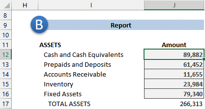
We would like to summarize the values. But, we would like to use different labels (or groups) in our report, like this:

Our data is presented by account, such as Checking account, Money market, and Savings. But these three values need to be summed and presented in the report line called Cash and Cash Equivalents.
So, one option is to include a mapping table in the workbook, which essentially provides Excel with the translations needed. It looks like this:

Now that we have told Excel how the account names (AcctName) translate into financial statement lines (FS Line), we need to write a clever formula to summarize the corresponding values for the report. So, let’s get to it.
Details
We will write our formula into the report, and it will retrieve and aggregate the corresponding amounts. We want to write our formula in the first report cell J12, and we want to be able to copy that same formula down for all report rows:

Our formula will use FILTER, SUMIFS, and SUM. Let’s talk through them one at a time.
Note: not all versions of Excel support the FILTER function. To determine if yours does, navigate to any blank cell and type =FIL. If you see FILTER in the drop-down function list then you are good to go. If not, use this technique instead.
FILTER
We will use the FILTER function to return a list of the accounts for any given fs line. For example, when we ask it to retrieve all accounts in the mapping table for Cash and Cash Equivalents, we want it to return Checking account, Money market, and Savings.
We write the following formula into J12:
=FILTER(Table2[AcctName],Table2[FS Line]=I12)
This tells Excel to retrieve the values from the AcctName column, where the FS Line column value is equal to our report line in cell I12. Since the formula returns multiple values, Excel automatically uses the adjacent cells to display those values. So, the single formula in J12 returns three values, which are displayed in the spill range J12:J14 shown below:

We can see that our formula successfully returned the three accounts that are mapped to the Cash and Cash Equivalents fs line. So far so good … now we need to somehow add the amounts for those accounts. This is where SUMIFS will come in handy.
Note: if the cells in the adjacent spill range are occupied, you’ll receive a #SPILL! error until you clear those cells. If you’d like to learn more about the FILTER function, check out this post.
SUMIFS
We will use the SUMIFS function to add up all of the rows in the data table for each of the accounts returned by the FILTER function.
So, we update our formula in J12 as follows:
=SUMIFS(Table1[Amount],Table1[AcctName],FILTER(Table2[AcctName],Table2[FS Line]=I12))
You’ll notice that we basically used the previous FILTER function as the third argument of the SUMIFS function. This tells Excel to add up the values in the Amount column, but only include those rows where the AcctName value is equal to the accounts returned by the FILTER function.
The results are shown below (these are the amounts for the three individual Cash and Cash Equivalents accounts):

Now, we just need to aggregate the three results into a single value, and we’ll do it with the SUM function.
Note: if your data table contained only one row for each account, you could use XLOOKUP instead of SUMIFS. The benefit of SUMIFS is that it works even when there are multiple data transactions for each account.
SUM
The final step is to add up all of the values returned by the SUMIFS function. We can do this by wrapping a SUM function around our previous formula, like this:
=SUM(SUMIFS(Table1[Amount],Table1[AcctName],FILTER(Table2[AcctName],Table2[FS Line]=I12)))
We hit enter, and bam:

Now we can just copy or fill that formula down for the remaining report rows, and we are good to go:
Conclusion
The idea of using a mapping table to translate labels is very helpful. There are many ways to implement a mapping table, and this post demonstrates one such option. The benefit of this option is that it doesn’t require a helper column. I really hope this article helps 🙂
If you have any thoughts, comments, questions, or alternatives, please post a comment below!
Sample file
Excel is not what it used to be.
You need the Excel Proficiency Roadmap now. Includes 6 steps for a successful journey, 3 things to avoid, and weekly Excel tips.
Want to learn Excel?
Our training programs start at $29 and will help you learn Excel quickly.
A great example of mapping process and table.
I found this blog and sample file very helpful.
Not sure I’ve understood this properly. Why wouldn’t you just use SUMIF to look for all specific categoroies like Cash and Cash equivalents. Why add the Filter and SUM bits?
I wondered the same thing – SUMIFS will do this without Filter.