Interest Payment IPMT

If you’re managing loans or curious about how much interest you’re paying each month, Excel’s IPMT function is here to help. In this post, we’ll not only explore how the function works, but we’ll also take it further by building a fully dynamic loan amortization schedule—one that updates automatically when you change any loan inputs. Let’s walk through it step-by-step.

Video

What is the IPMT Function in Excel?

The IPMT function in Excel calculates the interest portion of a loan payment for a given period. It works alongside its counterparts like PMT (for total payment) and provides incredible utility when we need to break down payments into interest and principal components.

Syntax:

=IPMT(rate, per, nper, pv)

• rate – Interest rate per period (annual rate divided by 12 for monthly loans).
• per – The specific period (e.g., month 1, month 2).
• nper – Total number of periods (months).
• pv – Present value or loan amount.

Step-by-Step: Create a Loan Interest Calculator with IPMT

Step 1: Define Loan Parameters

We’ll start with the basics. Set your spreadsheet like this:

• Loan Amount (C7): 10,000
• Loan Term in Months (C8): 12
• Annual Interest Rate (C9): 5%

Then, let’s calculate the total monthly payment in C10 by using the PMT function:

=PMT(C9/12, C8, -C7)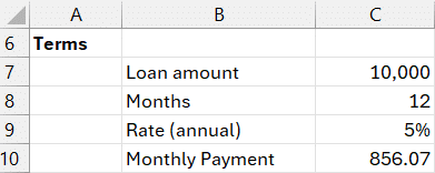

Output: 856.07 – This is the total amount paid each month.

Step 2: Calculate Interest for a Specific Period

Now, let’s determine how much of that $856.07 is interest in the first month. Use in C14:

=IPMT(C9/12, C13, C8, -C7)

This tells us that of the total payment of 856.07, 41.67 goes to interest (and the balance to principal).

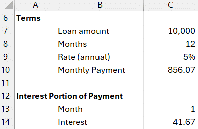
We can type different month numbers into C13 and instantly see the corresponding interest payment for that period.

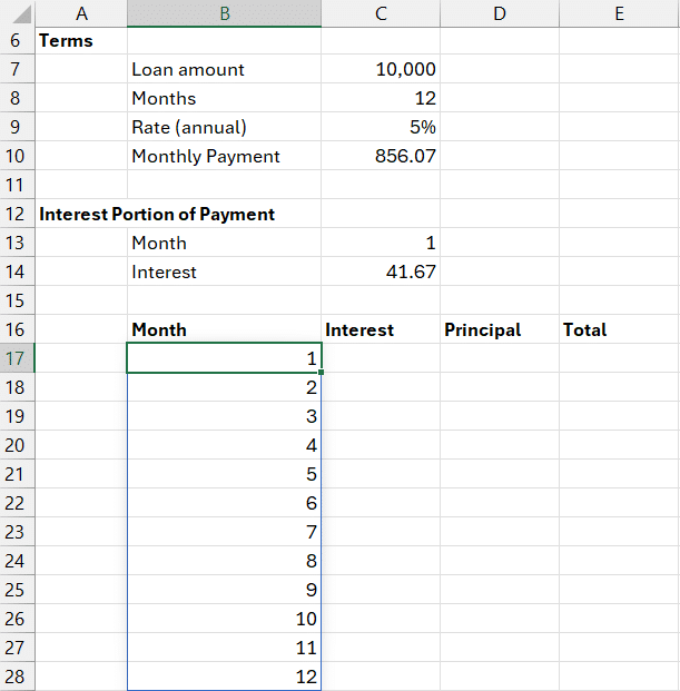
Step 3: Build a Dynamic Loan Amortization Schedule

Instead of changing each month number manually, let’s list them dynamically using the SEQUENCE function in B17:

=SEQUENCE(C8)

This creates a vertical list from 1 to 12 (or any loan term you specify in C8).

Step 4: Add the Interest Column

In column C (starting at C17), calculate the interest per month using a spilled range:

=IPMT(C9/12, B17#, C8, -C7)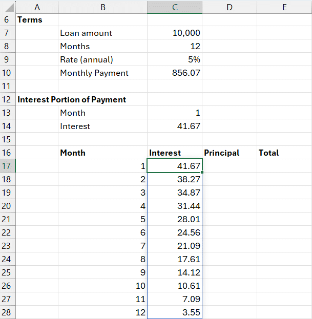

Step 5: Add Principal and Payment Columns

Still using our spilled ranges, let’s calculate the monthly principal now. We’ll subtract the total monthly payment from the interest for each month in D17:

=C10-C17#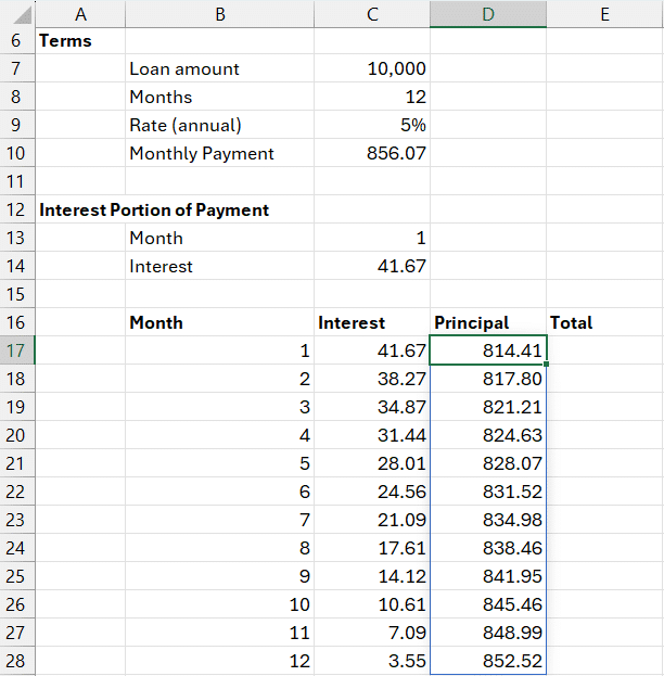

Finally, let’s add a total payment column:

=C17# + D17#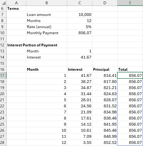

Step 6: Add Totals

To sum all three major columns, we can use the following formulas in F7, F8, and F9:

• Total Interest: =SUM(C17#)
• Total Principal: =SUM(D17#)
• Total Paid: =SUM(E17#)

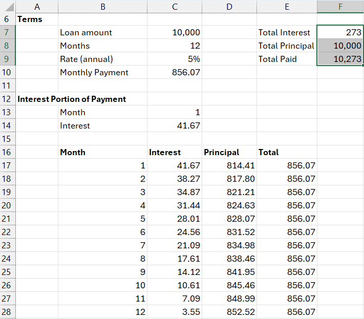
Everything is now 100% dynamic. Change the number of months, adjust the interest rate, redo the loan amount—your schedule updates automatically.

Summary

The IPMT function in Excel is a powerful tool for analyzing loan interest over time. When combined with PMT, SEQUENCE, and spill formulas, it helps us build a robust, dynamic amortization schedule. All we need are a few formulas, and we unlock a deeper understanding of how loans work and how payments are split between interest and principal.

With just a few formulas, we’ve created a comprehensive, dynamic, and scalable loan payment schedule. Keep exploring and take full advantage of Excel’s financial functions!

Download the Example File

Frequently Asked Questions

1. What does IPMT stand for in Excel?
   Interest Payment – it calculates the interest part of a loan payment for a specific period.
2. Why is the IPMT result negative?
   Excel treats loan payments as cash outflows, hence returns negative values by default.
3. How is IPMT different from PMT?
   PMT gives the total payment, while IPMT gives only the interest portion.
4. Can I calculate principal with IPMT?
   Yes, subtract interest (IPMT) from the total payment (PMT) to get the principal component. Alternatively, use the PPMT function.
5. What happens if I change the loan term?
   If you’re using SEQUENCE and spilled ranges, everything will update automatically.
6. Is this method suitable for variable interest loans?
   No. This setup assumes a fixed interest rate over the loan term.
7. Can I use this for credit card calculations?
   Not directly, as credit cards often have compounding and varying balances. This is for loans with a constant rate and payment.
8. Why use dynamic arrays and SEQUENCE?
   They make the schedule responsive and reduce manual inputs and formula dragging.