Impossible PivotTables 4 – Average of Distinct Count

This is the 4th and final post in the Impossible PivotTables series, where we are exploring Power Pivot by looking at some limitations encountered with traditional PivotTables. In this post, we’ll look at how to compute the average when there are multiple rows per item. That is, where a simple sum divided by the count of rows isn’t sufficient, and instead, we need to divide the sum by a distinct count of the number of items. For example, when we want the order averages, but, our data has multiple lines per order. Let’s get to it.

Objective

Before we get to the techie stuff, let’s just confirm our objective.

Let’s take a look at a portion of the data table:

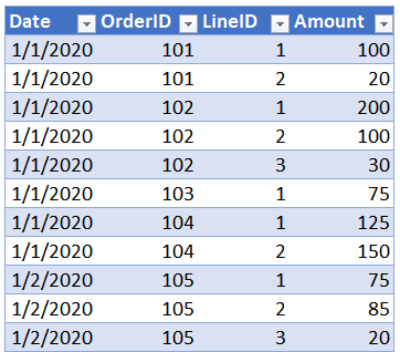
In looking at the data table, we see there can be multiple orders per day, and that each order can have multiple lines. For example, order 101 has two lines (rows), and order 102 has 3 lines.

We would like to know the daily average order amount. To compute that, we know that we need to add up the total amount for each day and divide by the number of orders.

Let’s try this with a traditional PT first. When we insert the Date and Amount fields, we see the sum as expected:

Then, we right-click any value in the Sum of Amount column and select Summarize Values By > Average. The updated PT is shown below.

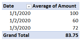
The PT displays an average, so, we think we are good to go. Or…are we? Upon closer inspection, we can see that the PT average is simply the sum divided by the number of data rows. For example, on 1/1/2020 the sum is 800 and the total number of rows (order lines) is 8. So, our PT displays 800 divided by 8, or 100. But, that isn’t the average we are looking for. We are looking for the average order, not order line. Hmmm.

The numerator (sum) is correct. But, the denominator isn’t what we are looking for. The denominator is the number of rows rather than the number of orders. These two values are not the same because there are multiple data rows per order. Drats. We hit a limitation and now we are stuck. Or…are we? As you may suspect, this is exactly where Power Pivot comes to our rescue.

Overview

We’ll compute the average order amount per day as follows:

• Load the data model
• Set up the basic PT
• Write the measure

Let’s get to it.

Note: The steps below are presented with Excel for Windows 2016. If you are using a different version of Excel, please note that the features presented may not be available or you may need to download and install the Power Pivot Add-in.

Load the data model

To load the table into the data model, we click any cell in the table and use the Power Pivot > Add to Data Model command. The Power Pivot window confirms the table is in the data model as shown below.

With our table in the data model, it is time to get our basic PT started.

Set up the basic PT

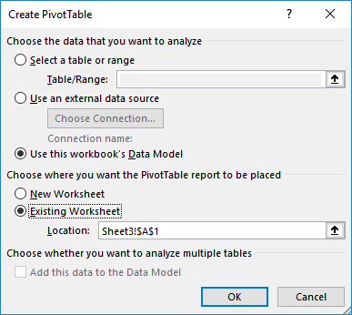
We use Excel’s Insert > PivotTable command, and confirm we opt to Use this workbook’s Data Model as the source, as shown below.

We then insert the Date field into the Rows layout area and the Amount field into the Values area. The basic PT is shown below.

At this point, it displays the same values as the traditional PT. It is now time to write a measure to compute the desired average.

Write the measure

We use Excel’s Power Pivot > Measures > New Measure command to open the Measure dialog. The measure name will be AvgOrder, and the formula will divide the Sum of the Amount by number of orders, as shown below.

Let’s break the formula down. We use the DIVIDE function to perform the division. The first argument is the numerator, which is the [Sum of Amount]. The second argument is the denominator, which uses the DISTINCTCOUNT function to count the number of unique orders in the OrderID column.

We click OK, and the PT is updated, as shown below.

Now, let’s just double-check the math to be sure we got it. For 1/1/2020, the total amount is 800, which looks good. By inspecting our table, we see that there are 4 orders for that day, and so 800 divided by 4 is 200 … yes, it worked! And, we see there is 1 order for 1/2/2020, and 180 divided by 1 is 180 … perfect! There are 3 orders on 1/3/2020, and 360 divided by 3 is 120 … great! And let’s just double-check the grand total. We see there are 8 orders in total, and 1340 divided by 8 is 167.50 … I think we got it!

If you have any other Power Pivot advice, please share by posting a comment below…thanks!

Sample File:

• AvgDistinctItems.xlsx