Impossible PivotTables 3 – Multiple Data Tables

This is the 3rd post in the Impossible PivotTables series. This series is designed to explore Power Pivot. I thought looking at a few limitations of traditional PivotTables would be a fun way to do this. So, in this post, we will look at how traditional PivotTables support a single data table while Power Pivot supports multiple data tables.

When we have multiple data tables and want to build a traditional PT, we end up with some sort of workaround. For example, we may merge the tables together to create one big data table, either by appending them (stacking them one after the other) or using formulas to retrieve related values, such as with VLOOKUP or other functions. The issue with this workaround is that we have to perform the same preparation steps each period. That is, the update isn’t a quick click of the Refresh command, it is a series of unfortunate tasks. Well, as you may suspect, this is where Power Pivot can help because it supports building PivotTables from multiple data tables. Let’s dig in.

Objective

Let’s suppose that our company creates an annual budget. As we go through the year, we also create a monthly forecast which reflects changes and updated business information. Plus, we record actual data which is available each month after our monthly close.

The budget data is stored in our budgeting application, the forecast data is stored in a custom application, and our actual data is stored in our accounting system. We need to build a report that compares the budget to the historical actuals plus projected forecast. That is, we need to use actuals when they are available, and forecast data when actuals are not yet available. For example, if we are in the month of December, we need to compare the annual budget to the Jan-Nov actuals PLUS the Dec forecast. We need to build one report that incorporates values from three different places.

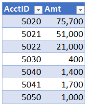
So, we get to work and export the budget data and save it in an Excel table named Bud, as shown below.

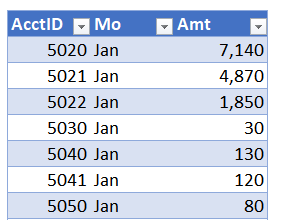
We export the monthly forecast data, and save it an another Excel table, named FC, as shown below.

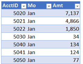
We export the monthly actuals, and save it in another Excel table, named Act, as shown below.

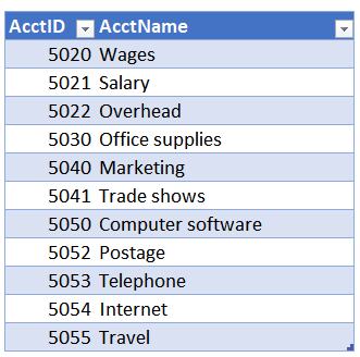
Oh yeah, we also have a chart of accounts, so we export that and save it in a table named Accounts, as shown below.

Now, we have an Excel workbook with 4 tables and we want to summarize them with a PivotTable.

Since a traditional PT supports but a single data table, we prepare to combine four tables into one. We begin by creating helper columns in the data tables that use VLOOKUP to retrieve the account name from the Accounts table. Then, we copy/paste append the three data tables that store budget, forecast, and actuals so they are all stacked up. This proves to be rather time-consuming because the columns don’t exactly line up. Plus, we lose track of which rows represent budget, actual, and forecast, so, we add another helper column that identifies the source of each row, as budget, forecast, or actual.

Now that we have combined these tables into one great big table, we begin to summarize it with a traditional PT. But, we soon get stuck. It is December, so, we have actual data through November. Our report needs to include Jan-Nov actuals, and Dec FC. We try to use a calculated field to do this. But, we quickly realize that calculated fields are good for basic math, but, aren’t really designed for this type of thing. As you may have guessed, Power Pivot is. Plus, if we use Power Pivot, we won’t need to go through the steps of setting up helper columns, using VLOOKUP to get the account names, or aligning and stacking the tables to create one big table. Power Pivot supports multiple data tables. Let’s see how we can build this report with Power Pivot.

Overview

We’ll create our PT using these steps:

• Load the tables into the data model
• Get the basic PT working
• Write the measures

Let’s get started.

Note: The steps below are presented with Excel for Windows 2016. If you are using a different version of Excel, please note that the features presented may not be available or you may need to download and install the Power Pivot Add-in.

Load the tables into the data model

First, we need to load the four tables into the data model. To do so, we select any cell in the desired table and use the Power Pivot > Add to Data Model command. We do this once for each table.

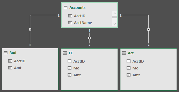
With the tables loaded, we need to create the relationships on the AcctID column. To do so, we use Power Pivot’s Home > Diagram View command, and then click-and-drag the AcctID column from each of the data tables into the Accounts lookup table. The resulting diagram view is shown below.

With our tables loaded into the data model and related, it is time to get our basic PT working.

Get the basic PT working

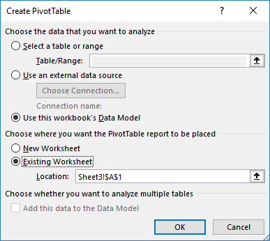
We use Excel’s Insert > PivotTable command and opt to Use this workbook’s Data Model in the resulting dialog, as shown below.

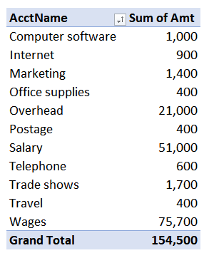
We then insert the Accounts[AcctName] field into the rows layout area and the Bud[Amt] field into the values area. Our basic PT is shown below.

Now, it is time to write the measures.

Write the measures

First, we’ll create a measure that computes the sum of Actual data for Jan-Nov and FC data for Dec. We’ll call this measure ActFC. We use the Power Pivot > Measures > New Measure command and write the corresponding formula into the dialog, as shown below.

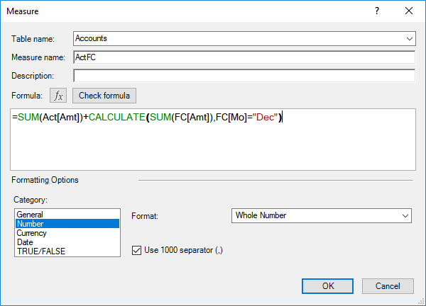
The formula essentially adds the actual data for all months in the table to the December FC data. Here is how the formula breaks down. The first part, SUM(Act[Amt]) computes the total of the actuals. The second part uses the CALCULATE function to add the forecast data for Dec only. The first argument of CALCULATE, SUM(FC[Amt]), tells the function to add up the forecast table’s amount column. The second argument, FC[Mo]=”Dec” tells it to only include those rows where the month is equal to December. This is similar to Excel’s SUMIFS function here, where we add up a column of numbers, but only include certain rows.

Up next is the variance, which is just the difference between the budget and the ActFC value. So, we write the following measure.

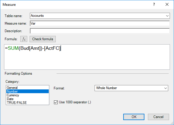
We add the measures to the report and enter our desired report labels. The updated report is shown below.

Now, the only little cosmetic detail we need to address is the sort order. Currently, the report is sorted in AcctName order. But, we’d like it presented in financial statement order, that is, account number order. To do this with a traditional PT, we would need to include the account number field, create a custom list, or manually click-and-drag the account rows. Let’s see how we do this with Power Pivot.

In Power Pivot, we select the Accounts table, and then select the AcctName column. We click the Home > Sort by Column command.  In the resulting dialog, we tell Excel to sort the AcctName column by the values in the AcctID column, as shown below.

We head back to view our PT, and yes … it worked!

If you have any other fun Power Pivot tips, please share by posting a comment below.

Also, feel free to check out the sample file below.

Sample file

• Multiple Data Tables.xlsx