How to Count Cells That Contain Specific Text

Have you ever wanted to see how many times a certain text string pops up in a set of data? While you can use Ctrl + F to find values, you may need a search feature that’s more discerning and responsive.  Luckily, there are several (much faster!) ways you can count cells that contain specific text in Excel.

Using Excel’s COUNT Functions

Several counting functions are available in Excel:

• COUNT – Counts how many cells contain numbers
• COUNTA – Counts the number of non-empty cells
• COUNTIF & COUNTIFS – Counts cells that meet specific criteria
• COUNTBLANK – Counts the number of blank cells

To see how they work, let’s say you’re responsible for buying fruits for a vendor, and you want to see how many cases of apples you have in stock.

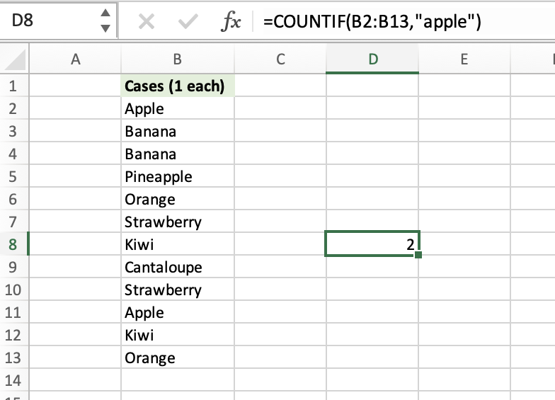
We can use the COUNTIF function to count the number of cells that are equal to apple (case insensitive). If we wanted to type the search value apple directly into the formula: 

=COUNTIF(B2:B13,"apple")

Or, if we wanted to refer to a cell (such as B2) that contained the value apple instead:

=COUNTIF(B2:B13, B2)

Note: COUNTIF evaluates one condition; if you need to count cells based on multiple conditions use COUNTIFS instead.

You’ll notice that this counts the cells that match apple. It does not count the number of times the word apple appears. In other words, a cell must only contain the word apple to be included in the count. For example, any cells containing the value pineapple or red apple would be excluded.

So, the next logical question is: what if we DO want to count cells that include apple anywhere within the cell? That is, what if the cell contains a partial match such as pineapple or red apple? To count cells that include a partial match, we can use wildcard characters.

Using Wildcard Characters to Count Cells that Contain Specific Text

Excel’s wildcard characters are unique symbols that can be used in formulas to represent other characters. They’re used to find matches that follow a defined pattern.

The wildcard symbols are:

• Question mark (?) – Represents one single character. For instance, ?n could match in or on.
• Asterisk (*) – An asterisk stands for an undetermined number of characters. Be*, for instance, could refer to behind, before, between, and so on. 
• Tilde (~) – Finds wildcard characters in a text string. More on this below.

We can use these wildcards to perform partial matches. That is, where we count cells that include specific text even if the cell includes other characters as well.

Using the Question Mark Wildcard Character

The question mark (?) wildcard represents a single character in a text string. You can use several question marks to represent a specific number of characters, for example:

=COUNTIF(B2:B13,"b???na")

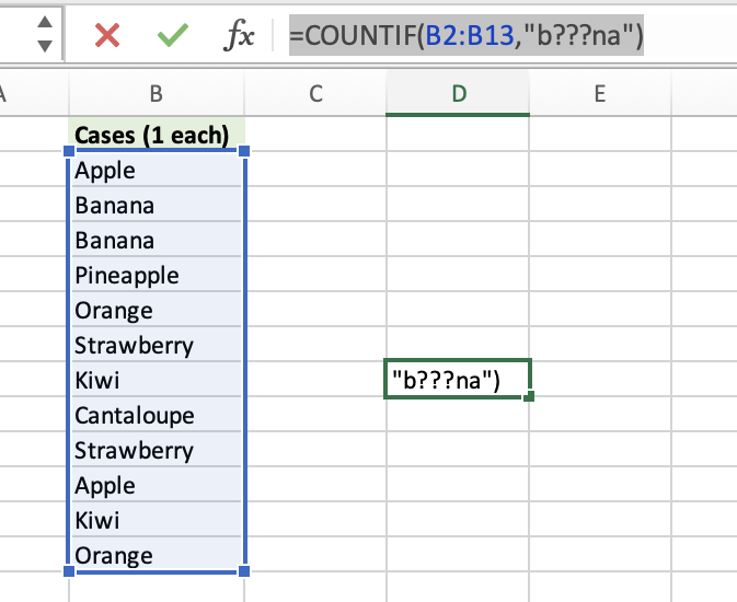
This will match values that starts with b, then includes exactly 3 other characters, then ends with na. In our case, it would match 2 cells since banana is the only value in our list that meets the match criteria.

If you want to count the number of cells that contain a text string of a specific length, you could repeat ? a given number of times. For example, to count the number of cells that contain a text of length 4:

=COUNTIF(B2:B13,"????")

And so on!

Using the Asterisk Wildcard Character for a Partial Match

We mentioned earlier that designating the value apple will count cells that only contain apple (no more or less characters). But, what if you want to include cells that contain the text string apple anywhere within the cell?

To do that, we’re going to use the asterisk wildcard character in a formula like this:

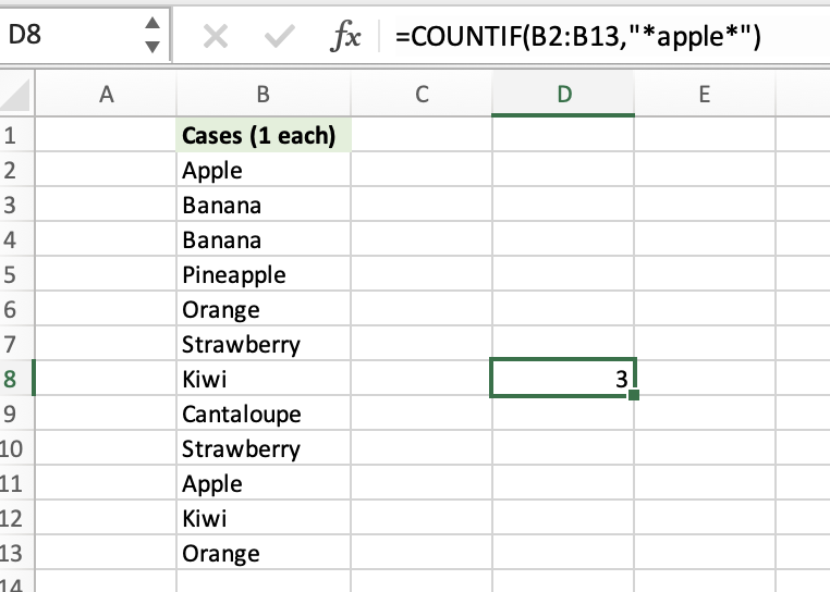
=COUNTIF(B2:B13,"*apple*")

Or, if we wanted to refer to a cell (B2) that contained the search term apple, we could join the wildcards with the cell reference like this:

=COUNTIF(B2:B13, "*"&B2&"*")

This will count the cells that start with any number of characters (including no characters), followed by apple, followed by any number of characters (or no characters). In our case, the number of cells counted increased to three. That’s because the asterisk (*) wildcard matches an undetermined number of characters before and after the word apple, so pineapple is now included in the count.

Note that you can modify the placement of the asterisk as desired. For example, *apple would match any text string that ends with apple, and apple* would match any text string that begins with apple.

Counting Empty and Non-Empty Cells

To count the total number of non-blank cells in a range, you could simply use the asterisk in a formula like this:

=COUNTIF(B:B,"*") 

Or, you could use COUNTA to count non-empty cells, like this:

=COUNTA(B:B)

Alternatively, if you wanted to count the empty cells:

=COUNTBLANK(B:B)

Now, let’s circle back to that tilde ~ character.

Using the Tilde Character

The tilde enables us to search for the wildcard character (instead of treating the character as a wildcard). In other words, if you wanted to tell Excel to look for the asterisk instead of treating the asterisk as a wildcard. For example, let’s say you need to locate the exact word kiwi*.

Any string that starts with kiwi would be returned if you used the string kiwi* (such as kiwifruit). This is because Excel would see the asterisk and use it as a wildcard. We can precede the asterisk with the tilde to prevent this behavior.

So, to specify the literal string kiwi*, we can use kiwi~* like this:

=COUNTIF(B2:B15,"kiwi~*")

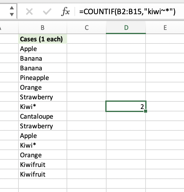
The tilde makes sure that Excel recognizes the asterisk as a part of the text string and not as a wildcard character.

How to Count Cells that Contain Specific Text – Case Sensitive

The COUNTIF method above won’t work when you need to perform a case sensitive search. That is, when you want to distinguish between uppercase and lowercase characters. Instead, you can combine the SUMPRODUCT and EXACT functions to count the number of cells containing case sensitive text:

=SUMPRODUCT(--EXACT("text", range))

The two hyphens in the formula convert the TRUE and FALSE values (returned by the EXACT function) to 1 and 0 respectively. The SUMPRODUCT function then sums these results and provides the total number of cells that match. 

Note: you can use the N function instead of the two hyphens to convert TRUE/FALSE to 1/0 if desired.

To put it into practice, let’s match the lowercase value in cell B2 (apple):

=SUMPRODUCT(--EXACT(B2, B2:B14))

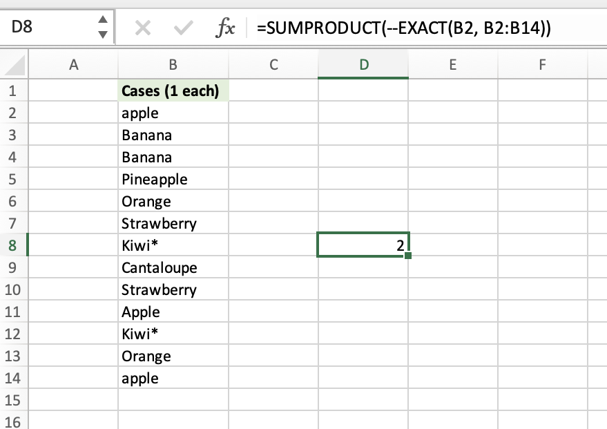
The formula returned a count of 2. It included cells B2 and B14 (lowercase apple), and it didn’t include cell B11 (Apple with an uppercase A).

Partial Match – Case Sensitive

To perform a partial match that is case sensitive, we can use the following formula:

=SUMPRODUCT(--ISNUMBER(FIND("text",range)))

The case sensitive FIND function returns an array of numbers (if the text is found in the range) and errors (if the text is not found in the range). The ISNUMBER function then converts the numbers to TRUE and errors to FALSE. The double negative converts TRUE/FALSE values to 1/0 values. Then, the SUMPRODUCT function sums the results and provides the total number of cells.

Here’s how the formula looks in action:

=SUMPRODUCT(--(ISNUMBER(FIND(D2, B2:B14))))

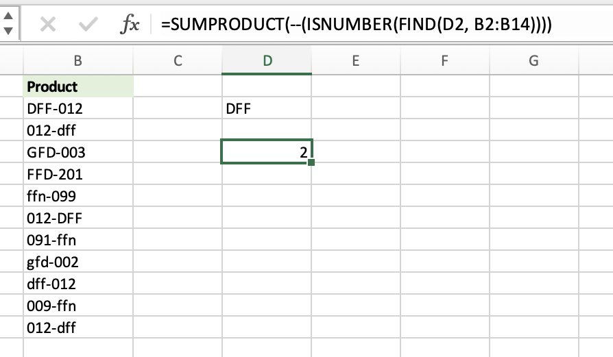
The formula counted the number of cells where uppercase DFF (case sensitive) matched anywhere within the cell value (partial match). 

These formulas can be fun to experiment with, and they come in handy when you’re sorting through large amounts of data. 

Do you have any other tips for quickly counting specific cells? Let us know in the comments!