How to Build a PivotTable with the Data Model

Traditional PivotTables are an incredible feature of Excel, but, they are not without limits. Many of the typical restrictions are removed when you use the data model rather than a single Excel table. If you’d like to learn how to build a PivotTable using the data model, and learn what the data model is, strap in…this will be a fun post.

Overview

Before we get too far, let’s jump up to 30,000 feet. For starters, what exactly is the data model? The data model provides a way to organize tables and formulas that can be used in a PivotTable. The data model comes with Excel 2016+ for Windows, and was formerly available as the Power Pivot add-in. The remainder of this article is presented with Excel 2016 for Windows.

Building a PivotTable from the data model rather than a single Excel table offers numerous advantages. Here are just a few to get us started.

• We can create a PivotTable that uses various fields from multiple tables.
• The formulas we can write far surpass those available in a traditional PivotTable. A language called DAX is used to write the formulas, and it provides many powerful functions.
• We can pick and choose rows and columns using named sets.
• We can directly connect to the data source (instead having to copy/paste data into a worksheet), use a Get & Transform query (to clean the data before it arrives), and connect to multiple data sources (eg, a csv file, a database table, and an Excel workbook) in a single model.
• Once built, we can just Refresh the report in subsequent periods (rather than having to go through the whole export, clean, import, and merge into a single data table process).

And, these are just a few of the highlights.

In this post, we are going to get warmed up by building a PivotTable from two tables. I’ve created a video and a full narrative with all of the step-by-step details below.

Video

Details

Our plan is to create a PivotTable from two tables. One data table has the transactions, and another table stores the chart of accounts. Historically, we would need to use VLOOKUP or something to first combine these tables into a single table to use with a traditional PivotTable. Here, we’ll use the data model. We’ll walk through these steps together:

• Enable the data model
• Import the data tables
• Define relationships
• Build the PivotTable

Let’s get started.

Enable the data model

First, we’ll need to enable the Power Pivot add-in. If you have Excel 2016+ for Windows, just click the Data > Manage Data Model ribbon command as shown below:

Note: depending on your screen size, you may see the icon only and not the label.

Clicking it the first time asks you to enable the add-ins:

Once you click Enable, you are all set and should see a Power Pivot ribbon tab. Yay!

Note: If you are on an earlier version of Excel for Windows, you’ll need to download and install the free Power Pivot add-in from the Microsoft website and follow the installation instructions for your version of Excel.

Import the data tables

Next, we import the data tables. In our case, we have some transactions stored in a DataTable workbook. The transactions have the account number but not the related account name. Fortunately, we have a little something called a chart of accounts, which is stored in the LookupTable workbook.

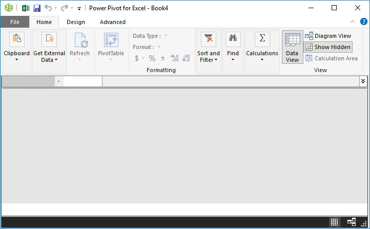
The step to import data tables will vary depending on where your source data is. To get started, click the Power Pivot > Manage ribbon command. This opens the Power Pivot window, shown below.

Use the Get External Data command to point to the underlying data source.

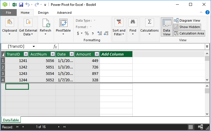
In our case, the data is in a couple of Excel files, so, we use the Get External Data > From Other Sources option, and then select Excel File in the resulting dialog. We Browse to the desired workbook and check Use first row as column headers. We finish the wizard and bam, the data is loaded into our data model, as shown below.

Note: if you are creating a data model inside the workbook that has the tables, you can use the Power Pivot > Add to Data Model command instead. 

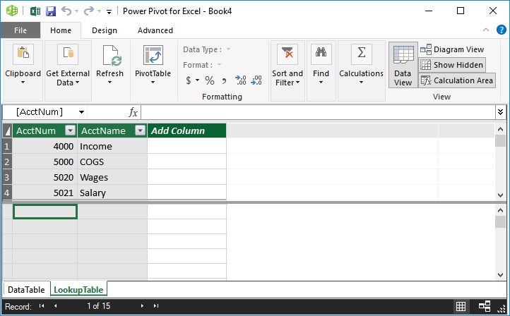
Next, we do the same thing to pull data from the LookupTable Excel file. The updated Power Pivot window is shown below.

With our data loaded into the data model, we need to tell Excel how the tables are related (which columns are common between the tables) by defining the relationships.

Define relationships

There are several ways to define relationships, but my favorite way is to use the visual diagram view. To toggle away from Data View (shown above), and Diagram view (shown below), simply click the Home > Diagram View command. We’ll now see the tables with the column names (instead of seeing the data transactions), as shown below.

To define the relationship, click the column name from the DataTable and drag to the related column in the LookupTable. In our case, we are relating the DataTable’s AcctNum column to the LookupTable’s AcctNum column. Excel displays the relationship as shown below.

With our relationship defined, we can now build the PivotTable.

Build the PivotTable

In the Power Pivot window, we just click the PivotTable > PivotTable command and select either a New Worksheet or an Existing Worksheet in the resulting Create PivotTable dialog. Once we click OK, bam, we see the familiar PivotTable field panel.

But, wait a sec … on closer inspection, it looks a little different from the traditional field panel. We typically see a list of fields that we can insert into the report. But now, we actually see the tables, and can expand each table to view the fields in each as shown below.

And, yes, we can pick fields from either or both of the tables for our report. For example, we want the AcctName from the LookupTable in Rows, and the Amount field from the DataTable as Values. And, bam … done!

Now, if your first reaction is that it would have been easier to just use VLOOKUP to create a single table, I totally understand. But, here’s the thing. This example is fairly simple because it includes but a single lookup table. The data model supports numerous lookup tables, for example, a chart of accounts, and calendar table, a department list, and so on. Plus, in addition to having multiple lookup tables in your data model, you can also have multiple data tables.

Plus, there is the issue of updating our report on an ongoing basis. Since we aren’t using VLOOKUP to retrieve related values, we don’t need to babysit a bunch of lookup formulas each month. As the external data source is updated, perhaps for a new account or new transactions, we can just Refresh and the new data flows into the report. As you can imagine, this opens up many interesting possibilities and can help save time in our recurring-use workbooks 🙂

Sample Files:

• DataTable.xlsx
• LookupTable.xlsx