Hide Rows in Excel Based on Cell Value (Without VBA)

Being able to hide rows based on cell value in Excel is a handy skill for anyone who needs to organize a large spreadsheet. Imagine you have a huge list of data, but only some of the rows are relevant to you at the moment. When you hide rows based on cell value, you can easily eliminate the rows that don’t matter and just focus on the data that does.

Here are a few ways to do it!

1. Using the Filter Feature
2. Using Conditional Formatting
3. Using Shortcuts to Hide Blank Rows
4. Data Outline to Hide Specific Rows

Use Excel’s Filter Feature to Hide Rows Based on Cell Value

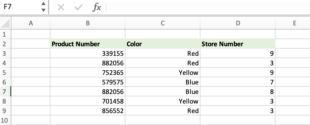
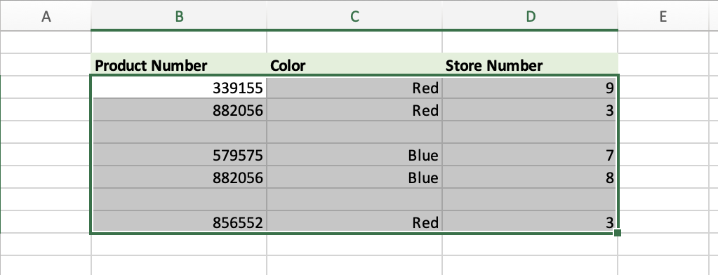
With Excel’s filter feature, users can hide rows, columns, or cells that don’t meet specific criteria. Let’s say you have a table like the one below containing information about certain products.

To use the filter feature, select any cell in the table and click Sort & Filter from the Home ribbon tab, then choose Filter. 

Click on any of the arrows that appear next to your column headings – in this example, we’ll filter the Color column.

The Filter command box will pop up, and you can simply deselect the items you’d like to hide along with their respective rows. We’ll hide the rows containing Yellow to get this result:

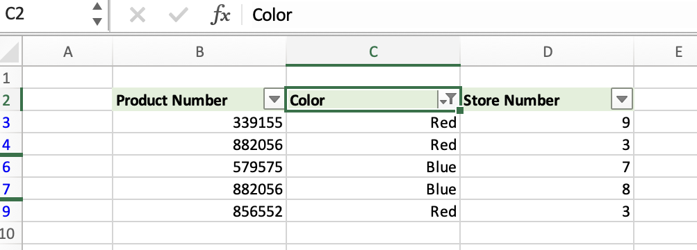
This is one of the easiest ways to hide rows based on a cell value, and the best part is that it works well no matter how large the dataset is.

How to Hide Rows with Conditional Formatting

What if you want to hide the content of the row, but still be able to see that a row is there? In that case, you’ll want to use conditional formatting to hide certain data. Here’s how to use it to hide the contents of some rows. 

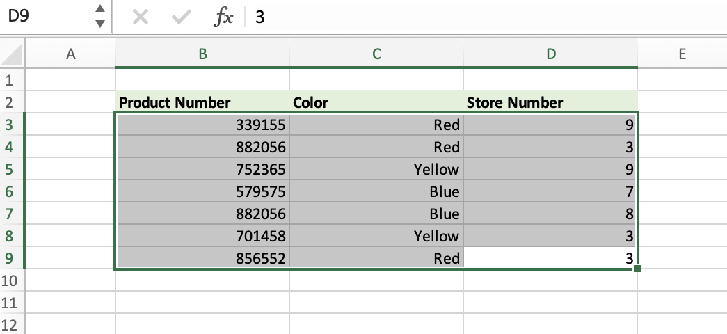
First, we’ll use the same table in the previous example. This time, you’ll want to select the entire table but exclude the headers. 

Navigate over to Conditional Formatting on the Home ribbon tab, select it, and choose New Rule. From the drop-down list, select Use a formula to determine which cells to format.

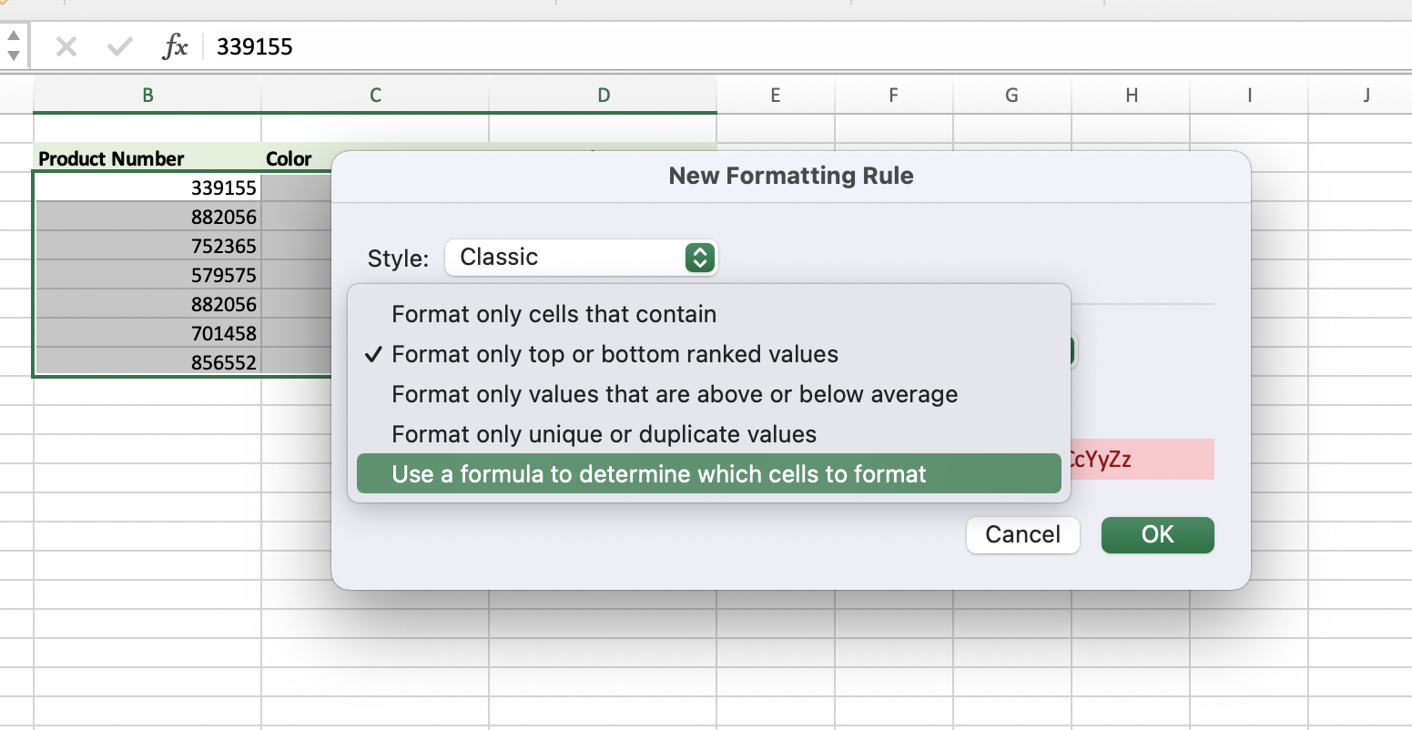
Type this formula in the formula bar:

 =$C3="Yellow"

Note: if you are writing a formula for your own workbook, be sure to update C to the column that has the value you are inspecting, and 3 to the row that contains the active cell. Be sure to include a $ before the column reference but not before the row reference.

Then choose Custom Format in the Format with drop-down menu, choose the Numbers tab, and select Custom at the bottom of the list. In the Type bar, enter three semicolons – “;;;” – and click OK.

You’ll see all the rows with a “Yellow” label in column C have been hidden from the grid!

One disclaimer here is that while the rows look blank, you can see the values by clicking the cells. So, this probably isn’t the best way to hide sensitive information if that’s the goal.

If you want to keep some info more private, see our post on how to hide formulas in Excel to learn more about controlling access to the formulas in your shared workbooks.

Hide Blank Rows in Excel Using Shortcuts

Ctrl + 9 hides any rows that are currently selected. Ctrl + Shift + 9 unhides them.

This can be useful if you have have a small amount of data to work with, but a lot of blank rows underneath. Hiding the blank rows can make it easier to see and work with the ones that do contain data.  To do it, select the first blank row after your data. For us, that would be row 10. Then use the shortcut Ctrl + Shift + Down to select all the empty rows, and Ctrl + 9 to hide them. Ctrl + Shift + 9 will unhide them.

Data Outline

You can also select a group of rows that you want to be able to quickly hide and then unhide. To do so, select the rows you want to group. Then click Data > Outline > Group. This will group the rows and provide an icon you can use to quickly hide them all. You can then click the icon again to unhide them all. To remove the outline group, select Data > Outline > Ungroup.

Sample File

---

Do you know any other easy ways to hide rows based on cell value in Excel? Let us know in the comments!