Get & Transform: An Alternative to VLOOKUP List Comparisons

I recently received an Excel question about how to perform a specific list comparison, and I thought I’d demonstrate how to use a Get & Transform query as an alternative to the formula-based list comparisons typically performed with functions such as VLOOKUP and COUNTIFS. The original question is: “I am trying to use a list of 79 credit card numbers to find all occurrences of each card number in a list of 400,000+ transactions. We are testing only transactions for those credit cards.” This type of list comparison can be performed with formulas, but in this post, we’ll use a Get & Transform query instead. Thanks Maria for your question!

Objective

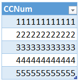
Before we get too far, let’s take a moment to visualize the data and our goal. The first list contains the credit cards selected for review. The table is named CreditCards and it looks something like this.

The second list contains all transactions. It is named Transactions and it looks something like this.

Our goal is to have Excel create a list of transactions for the CCNums that appear in the credit card list.

Now, if you only had a few card numbers, this task could easily be performed by using a filter. But, as the number of credit cards grows, this approach becomes more tedious and difficult to update in future periods. Another option would be to write a helper formula to the right of the transactions table. The formula could use a function such as VLOOKUP or COUNTIFS to see if each transaction’s credit card number appears in the credit card list. We could then apply a filter and call it good. Prior to Excel 2016, that is exactly the approach that I’d use, and I have an article referenced below that walks through the steps of the process. But, with the Get & Transform tools built-in to Excel 2016 for Windows, we have another option. Let’s see how to accomplish this task with a Get & Transform query.

Steps

We’ll proceed with the following steps:

• Create a connection to each list
• Create a merge query
• Return the results

Let’s do this thing.

Note: The steps below are presented with Excel for Windows 2016. If you are using a different version of Excel, please note that the features presented may not be available or you may need to download and install the Power Query Add-in.

Create a connection to each list

We need to create a connection to each list. First the list of selected credit card numbers. Select any cell in the table, and use the following Get & Transform command.

• Data > From Table

This opens the Query Editor, as shown below.

Note: We don’t need to worry about the format of the CCNum data, because the stored values are unchanged. 

Now, to create a connection rather than return the data to an Excel worksheet, we use the Close & Load To command (rather than Close & Load), by selecting the following command.

• Home > Close & Load > Close & Load To…

This displays the Load To dialog, where we select Only Create Connection, as shown below.

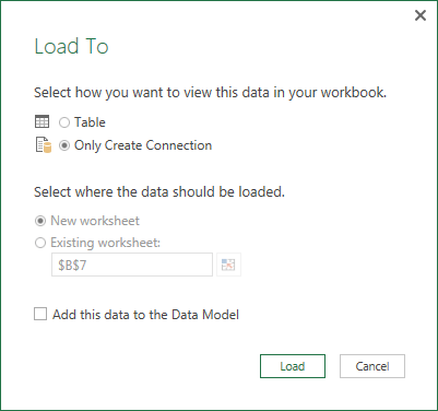
We click the Load button and now we have the connection only query. It is displayed in the Workbook Queries pane on the right of the Excel window, as shown below.

Now, we create another connection query for the transactions table, and we just use the same steps. Select a cell in the transactions table, use the Get & Transform From Table command, select Close & Load To, Only Create Connection, and Load. Now we have two connection queries, as shown below.

Now, we are ready to merge them.

Create a merge query

We can combine queries in two ways. We can “merge” them or we can “append” them. If we append them, we combine them vertically and sort of stack the two tables on top of each other. If we merge them, we combine them horizontally and sort of place the columns next to each other. This is what we would traditionally use VLOOKUP to accomplish. To create our merge query, we select the following command.

• Data > New Query > Combine Queries > Merge

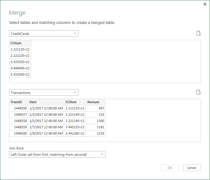
This brings up the Merge dialog box, where we can define how Excel should merge the two tables.

In our case, we want all credit cards in the credit card list, and only the transactions that match from the transactions table. So, we need to tell Excel that the first table is the CreditCards table, and the second table is the Transactions table as shown below.

Now we need to tell Excel which column should be used to match the tables. To do this, we select the desired columns from each table, in our case, it is the CCNum column as shown below.

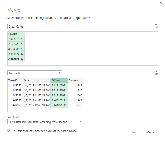
In our case, the join is technically called a Left Outer Join, which means it takes all records from the first table and only the matching records from the second table. There are other types of joins that are useful in other types of situations. We click OK to return to the Query Editor, as shown below.

At this point, we need to tell Excel to expand the new column and we need to identify which columns from the transactions table we want to display. We can do this either by clicking the little expand/aggregate button on the top-right side of the column label, or, by clicking the following ribbon icon:

• Transform > Structured Column > Expand

This displays the Expand dialog, where we can pick which transaction columns we’d like to include in the query results, as shown below.

We want all columns, so we just click OK. The column is expanded, and the results are displayed in the Query Editor, as shown below.

Wow! Now, all we need to do is return the results to Excel.

Return the results

To return the results to Excel, we use the Close & Load command. Bam….we have a new results table in our workbook as shown below.

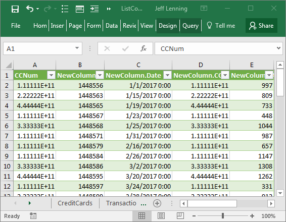
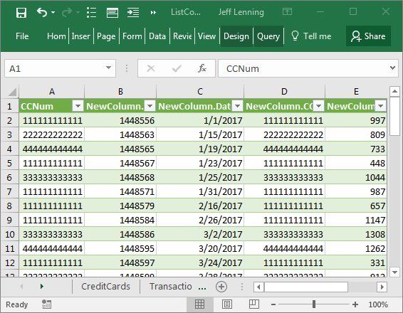
And, we can clean it up as desired, for example, by formatting the CCNum and date columns.

And the best part is that in future periods when either the credit card list or the transaction table is updated, we don’t need to go through these steps all over again…we just right-click the results table and refresh!

If you have any other fun list comparison or get & transform query ideas, please share by posting a comment below.

Resources

• Sample file: ListCompare
• Formula-based list comparisons article: Comparing Lists with Ease