Formula Override Conditional Formatting Alert
Let me ask you a question. How do you know when a user has entered a value into a formula cell, essentially overriding your formula? Since this is Excel, there are several ways to address this issue, but starting with Excel 2013, we can use conditional formatting with the new ISFORMULA function.
Objective
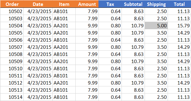
Our worksheet has a range of formulas. In the screenshot below, the orange columns contain values while the blue columns contain formulas.

Our goal is to change the formatting of the formula cell when the user enters a value, essentially replacing our formula with a static value. For example, if the user enters a different shipping amount, we want to format the cell fill with gray as shown for order 10504 below.
The good news is that beginning with Excel 2013, we can use the ISFORMULA function and a simple conditional formatting rule so that Excel automatically applies the desired cell formatting.
ISFORMULA
The first step is to understand the new ISFORMULA function. The ISFORMULA function was introduced in Excel 2013 and returns TRUE when the argument cell contains a formula and FALSE when it doesn’t.
For example, if A1 contains a formula, the following formula returns TRUE:
=ISFORMULA(A1)
In our worksheet, we want to format the cell when the cell does not contain a formula, so, we would actually want to apply conditional formatting with the following formula:
=NOT(ISFORMULA(A1))
The NOT function returns TRUE when A1 does not contain a formula, that is, it returns TRUE when a user entered a value into the cell.
Now, let’s set up the conditional formatting rule.
Conditional Formatting
To begin, we simply select the entire range of formula cells, in our case, the blue columns as shown below.
We take note of the active cell. You’ll notice that we selected the range F7:I19, however, only a single cell is active, F7. We make a mental note of this active cell, and then open the conditional formatting dialog with the following Ribbon icon:
- Home > Conditional Formatting > New Rule
In the New Formatting Rule dialog, we “Use a formula to determine which cells to format” and enter our =NOT(ISFORMULA(F7)) formula and reference the active cell (F7), as shown below.
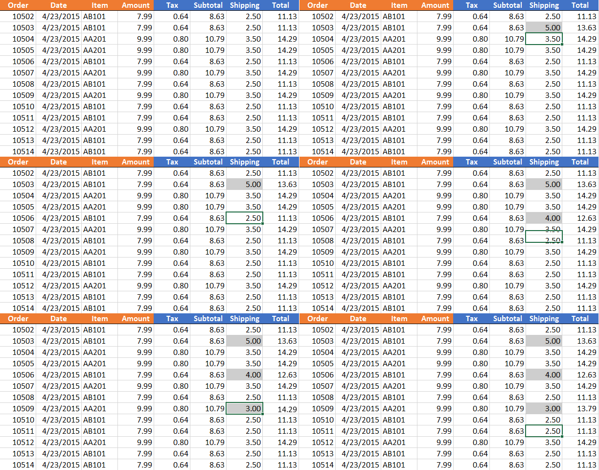
We select the desired cell formatting by clicking the Format button. Once we click OK and apply the rule to the selected cells, Excel will automatically format the cells whenever a user replaces a formula cell with a static cell value, as shown below.
And that is the ISFORMULA and conditional formatting method to address the issue. If you have any tips or alternatives, please share by posting a comment below…thanks!
Additional Resources
Excel is not what it used to be.
You need the Excel Proficiency Roadmap now. Includes 6 steps for a successful journey, 3 things to avoid, and weekly Excel tips.
Want to learn Excel?
Our training programs start at $29 and will help you learn Excel quickly.


I do not have Excel 2013 yet so I cannot test this – what happens if the user enters a formula which is really a constant because it does not refer to any other cells. In your example, I could see the shipping being made up of 2 pieces, postage and a flat handling charge and the user enters +3+2 instead of 5
Hiya Catherine!
To the ISFORMULA function, it would be considered a formula even if it doesn’t reference a cell and contains only an expression such as +3+2. If A1 contained +3+2 or =3+2, ISFORMULA(A1) returns TRUE.
Thanks,
Jeff
This is fantastic – I just read through almost a dozen sites that explained how this couldn’t be done, and you solution was simple, elegant, and effective! I was trying to put the range, rather than the active cell, in the formula – great to see how this issue can be resolved!
🙂
Is there a way, when using formula override conditional formatting, to have an error message come up (a pop up)
Yes…to do so you could apply Data Validation to the range (the same range as the conditional formatting). Then, change the Error Alert Style to Information. Then, when someone entered a value, the warning would pop-up but still allow the user to enter their value.
I have a blog post about Data Validation Error Alerts here: https://www.excel-university.com/data-validation-alert-styles/
Hope it helps!
Thanks
Jeff
Good Article!!!!
Would you be able to advise me on another issue I’m having,
I have an excel sheet to show me items that are due for delivery, so it will automatically highlight yellow if its due tomorrow or red if it is due today, in a column titled expected delivery
However, I am trying to have a function where this will only happen if there is no data in the ‘date delivered’ column, so is there a way I can set conditional formatting to either white (or not at all) in the ‘estimated delivery’ if there is a date entered into ‘Date delivered’?
Sorry if I’m confusing anyone!
Rob,
If you set up a conditional formatting formula, you could use AND to evaluate both conditions. That is, you would create one rule, using AND, to see if both the Date Delivered is 0 and Due is tomorrow. If so, it gets yellow. Another rule would use AND to see if both the Date Delivered cell is empty/0 and Due is today. If so, it gets red. This post talks about how to set up a conditional formatting formula:
https://www.excel-university.com/excel-conditional-formatting-based-on-another-cell/
Hope it helps,
Jeff