Find Last Occurrence

I was recently asked how to find the last occurrence of a value in a column. Although there are multiple ways to accomplish this, in this post, I’ll talk about how to use XLOOKUP.

Objective

Before we jump into Excel, let’s confirm our objective. Let’s say we have a bunch of transactions that look like this:

Now let’s say that we want to retrieve the Transaction ID for the last transaction for a given Item. For example, the last transaction for Item A is 1010. The last transaction for Item C is 1009. In other words, we want to start at the bottom and search up.

In this post, we’ll use our friend XLOOKUP.

Note: depending on when you are reading this, your Excel version may not have XLOOKUP. A quick way to determine if it does is to type =X in any cell and see if XLOOKUP appears in the resulting list.

Video

Narrative

XLOOKUP

XLOOKUP is designed to look for a matching value and return a related item. The basic syntax is:

=XLOOKUP(lookup_value, lookup_array, return_array)

There are also a few optional arguments, including one that enables us to define the search order. For example, first to last or … wait for it … last to first!

It is the 6th argument that enables us to define the search order. If we use 1 or omit it, it will search first to last. If we use -1, it will search last to first.

If we wanted to search last to first, our formula would look more like this:

=XLOOKUP(lookup_value, lookup_array, return_array, , ,-1)

Let’s give it a try.

Illustration

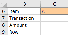
We type in the Item we are searching for in C6, and set up a few empty cells to store the Transaction, Amount, and Row, like this:

Let’s start by retrieving the last Transaction.

Transaction

To retrieve the Transaction ID, we write the following in cell C7:

=XLOOKUP(C6,C14:C23,B14:B23,,,-1)

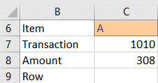
Since we used -1 for the 6th argument, the formula returns 1010:

Now, we can use the same technique to grab the Amount.

Amount

To retrieve the Amount, we write the following in C8:

=XLOOKUP(C6,C14:C23,D14:D23,,,-1)

The formula returns 308 … nice:

And … what about returning the row … can we do that?

Row

To get the row number, there’s one more thing about XLOOKUP to unpack. As we saw above, XLOOKUP returns a cell value … right? Seems like it.

But under the hood, it returns a range. When nothing else is going on in the formula, it simple returns the value from that range. But, we can use it with other functions as desired.

For example, the ROW function returns the row number of the argument. So, we can wrap the ROW function around the XLOOKUP function like this:

=ROW(XLOOKUP(C6,C14:C23,C14:C23,,,-1))

And it returns the row number of the last transaction for the specified Item:

Nice!

Bonus

Also, here is a little bonus. Let’s say we would like Excel to highlight the last transaction for the specified item, like this:

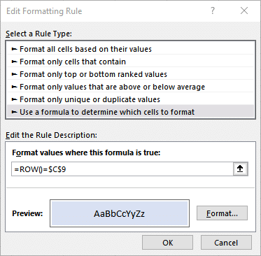
We can use Conditional Formatting to accomplish this. We can select the entire data range, in this case B14:D23 and select Home > Conditional Formatting > New Rule.

We select the Use a formula to determine which cells to format option, and enter the following formula:

=ROW()=$C$C9

We can then click Format to select our desired formatting.

Now, Excel will highlight the last transaction. So when we type in a new item, such as E, the worksheet updates:

As you can see, XLOOKUP offers a great way to find the last occurrence of an item in a column. Let me know what you think by posting a comment below. Also, if you have a preferred method or other option, please share it with others by posting a comment below … thanks!

Sample File