Find Cells That Contain Specific Text

The objective of this tutorial is to learn how to write formulas in Excel that can identify specific text strings within cells. We will start by using the SEARCH function to find cells that contain a specific word, then convert the results into TRUE / FALSE values, and finally apply conditional formatting to highlight these cells.

Video

Walkthrough

Let’s take it one exercise at a time.

Exercise 1: Using the SEARCH Function

Consider the following poem that I had ChatGPT write for me about Excel:

Let’s say that I wanted to identify the cells that contain the word “Excel.”

One option would be to write a formula in an adjacent column that uses the SEARCH function. For example, we could write the following formula:

=SEARCH(B9,"excel")

• B9 is the cell to search
• “excel” is the text to find (case insensitive)

Note: if you need the search to be case sensitive, use the FIND function instead of the SEARCH function.

We can fill that formula down, and bam:

As you can see, the SEARCH function returns an error when the word is not found, and a number when it is found. The number corresponds to the position within the cell that the text “Excel” is found.

But, what if we wanted to clean this up a bit? Like, instead of a bunch of errors and numbers, we wanted a clean TRUE/FALSE column. Well, that leads us to the next exercise.

Exercise 2: Converting Search Results into TRUE/FALSE Values

Starting with the same formula as the previous exercise, we’d like a way to change the results from errors and numbers to TRUE and FALSE. One option would be to the use ISERROR function.

The ISERROR function returns TRUE when the argument is an error, otherwise, it returns FALSE. This is the opposite of what we ultimately need, but, let’s take it one step at a time.

If we wrap the ISERROR function around our SEARCH function from before, the updated formula looks like this:

=ISERROR(SEARCH("excel",B9))

We fill the formula down, and we see:

Well … the output is much cleaner than the errors and numbers that we had before. However, this is the exact opposite of what we want. We want TRUE when the word “Excel” is found, but the results above show FALSE.

So, is there a way to basically flip the results? Where TRUE goes to FALSE, and FALSE goes to TRUE? Yes! One option would be to wrap the NOT function around the formula. So, the updated formula would look like this:

=NOT(ISERROR(SEARCH("excel",B9)))

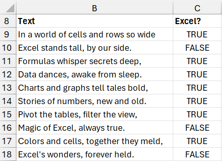
We fill this updated formula down, and bam:

Now, depending on what we are working on and our next step, this could be sufficient. We have a column that provides TRUE when the word “Excel” is found.

But, depending on what we are working on, we may want to somehow highlight the cells with some type of format, like cell fill, font, or border. Well, the good news is that we can easily use conditional formatting. Let’s do that now.

Exercise 3: Applying Conditional Formatting

First, we highlight the range of cells that contains the poem, or whatever cells contain the text you want to evaluate.

Then, we use the Home > Conditional Formatting > Highlight Cell Rules > Text that Contains command. In the resulting dialog, simply enter the word “Excel” and pick your desired formatting.

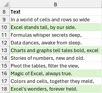
When we click OK, bam:

All of the cells that contain the word “Excel” are highlighted accordingly!

Conclusion

I hope this post provided helpful steps for writing formulas to identify specific text strings within cells. Plus, it showed how to convert the results into TRUE/FALSE values and how to apply conditional formatting to highlight the desired cells. If you have any improvements, questions, alternatives, or suggestions, please share by posting a comment … thanks!

Sample file

FAQs

Q: Can I search for case-sensitive words?

A: Yes … but instead of using SEARCH, you would use the FIND (which is case-sensitive).

Q: Can I apply conditional formatting to multiple ranges of cells?

A: Yes, you can select multiple ranges of cells and apply the same conditional formatting rule to all of them. Just make sure to select all the ranges before creating the conditional formatting rule.

Q: Is conditional formatting dynamic? Will it update automatically when I change the data?

A: Yes, conditional formatting is dynamic. It will update automatically when you change the data in the selected cells. The formatting will be applied or removed based on the updated conditions.

Q: Can I modify the formatting style after applying conditional formatting?

A: Yes, you can modify the formatting style of the conditional formatting rule at any time. Just select the cells and use the Home > Conditional Formatting > Manage Rules command.