Dynamic Arrays 1

During the years we have been using Excel, we have come to understand that a formula calculates a value. Meaning, a single value. Right? Like … we write a formula, hit Enter, and the result is displayed in the cell.

Easy … that is how we have been using Excel for decades.

Multiple Values

But … formulas can return multiple values (an array of values).

Historically, these types of array formulas were somewhat complicated to create and required pressing special keys to enter. As a result, many Excel users did not take advantage of them.

However … times have changed!

In the most recent versions of Excel, writing and managing such formulas is greatly simplified and no special keys are required. This makes it much easier to take advantage of these types of formulas.

Spill Range

But … hang on Jeff!

If I write a formula that returns multiple results, what happens? Does just the first result appear in the cell? Or what? Here’s how that works.

When you write a formula that returns multiple values (an array), the results spill out of the formula cell into the adjacent cells (called the spill range). Wait … what? Crazy … I know! And super cool. And, it gets even better.

If the number of results returned by the formula changes over time, the number of cells used to display the results changes accordingly. That is, it is dynamic. Thus the term Dynamic Array.

Dynamic Array Series

This is the first post in the Dynamic Arrays series where we’ll explore this concept. Hang on tight, it’s gonna be a wild ride 😉

Note: this capability is available at the time of this writing in Excel 365 subscription versions, and isn’t available in perpetual license versions of Excel such as Excel 2019, 2016, 2013, and so on.

Video

Functions that return multiple values

I know what you may be thinking right about now. What type of formula returns multiple results? I mean the functions I use all the time like SUM, AVERAGE, MIN, MAX, COUNT and so on compute a single value. It is hard to image a function that returns multiple values.

Well, there are several functions that are designed specifically to return multiple values … the first of which we’ll discuss is UNIQUE.

UNIQUE

The UNIQUE function is designed to return a list of the unique values found in a range. And there it is. It returns a list … that is … multiple values.

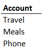
For example, let’s say we have a table named Table1 that looks like this:

And, let’s say we wanted to create a list of the accounts without any duplicate accounts. That is, we wanted to create a list like this:

To do this, we use the UNIQUE function. The argument is the Account column in our table:

=UNIQUE(Table1[Account])

When we type this formula, and press Enter … wow! That single formula actually creates the entire list:

We write one formula into a single cell. That formula returns multiple results. The first result is displayed in the formula cell and the remaining results spill out into the adjacent cells (the spill range).

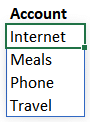
This spill range is dynamic … meaning if we add a row to Table1 that includes a new account, the new account will automatically appear in our account list that was created with the UNIQUE function. For example, if Table1 gets a new row for Internet, the formula dynamically updates the spill range accordingly, like this:

You’ll notice that the list of accounts is displayed in the order in which they appear in the data source. Travel is first, Meals second, and so on. What if we wanted to display our list in alphabetical order? Well, that leads us to our next dynamic array function, SORT.

SORT

The SORT function is designed to sort the range. The default sort order is ascending, but we have a few options and arguments if we want to get fancy. In our case, a simple ascending sort is what we are after, so we simply wrap the SORT function around our UNIQUE function, like this:

=SORT(UNIQUE(Table1[Account]))

When we press Enter … bam:

Again, this list is dynamic. So, when new accounts are added to the data table, our list of accounts is updated accordingly. Excellent!

Cool?

What do you think about this capability? Let me know by posting a comment below, thanks!

Sample file