Daily Bank Balance with a PivotTable

When you download banking activity, you typically get the transactions, but not the daily bank balance. To compute the daily bank balance, you need to summarize the transactions by day and display a running total for all days, even those without any activity. This post demonstrates how to build such a report using a PivotTable.

Overview

Before we dig into the technical details, let’s be clear about our objective. We have downloaded some banking activity and manually entered the beginning bank balance as of 1/1/2017. This is illustrated below.

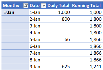
We’d like to build a report that displays one row for each day of the month, even if there are no transactions for that day. Plus, the report should show a running total that represents the daily bank balance. Essentially, we’d like to build a report that looks like this.

Let’s get to it.

Details

Building such a report can be accomplished with a PivotTable. I’ll walk through each step below. But, if you are already familiar with PivotTables, the short answer is this: group by month and day, show items with no data, and show values as a running total.

We’ll build this report using the following steps.

• Basic PivotTable
• Display all days
• Running total
• Cosmetics

Basic PivotTable

Let’s get the basic PivotTable set up. Select any cell in the data source range, and Insert > PivotTable. We place the report on a new worksheet and click OK.

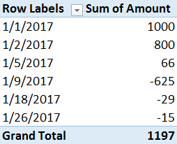
In the PivotTable Fields panel, we check the Date and Amount checkboxes. At this point, we have a basic PivotTable, as shown below.

Note: Excel 2016 for Windows automatically groups date fields, and if you are using a version prior to Excel 2016 for Windows, your report may look like this instead:

If it does, no worries, the steps below will work just fine 🙂

The biggest problem with our report is that it only displays days with activity. But, our report needs to include one row for every day of the month, even those without any transactions. So, the next task is to display all days.

Display all days

We want to display all days, even those without any data transactions. To do this, the date field needs to be grouped. We want our report grouped by month and day. So, we, right-click any date cell in the report, and select Group.

This displays the Grouping dialog, where we pick Months and Days, as shown below.

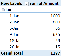
We click OK and our report now looks like this:

Now, we open the Field Settings dialog for the Date field (not the Months field). An easy way to do this is to right-click any day in the report, and select Field Settings. In the resulting Field Settings dialog, we head to the Layout & Print tab. There, we find a checkbox named Show items with no data. We check it, as shown below.

We click OK and wow! We now see one report row for each day, as shown below.

Note: if you group the date field by month, then you can show months with no data. If you group by day, then you can show days with no data. That is, the Show items with no data checkbox can be applied to the desired date group field.

We are getting closer! At this point, we need to add a running total column.

Running Total

Adding a running total column is not too bad. We begin by inserting the Amount column into the Values layout area again. An easy way to do this is to click-and-drag the Amount field into the Values area.

Now we have two Amount columns in the report. We’ll leave the first one as is, and we’ll convert the second Amount column into the running total. To do this, we right-click any value cell in the second Amount column, and select Show Values As > Running Total In. In the resulting Show Values As dialog, we accept the default base field (Date) and click OK.

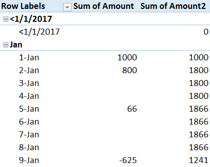
Bam, our report now includes a running total column, as shown below.

Our basic report is done, now we just need to clean it up and make it pretty.

Cosmetics

I’ll go ahead and summarize the steps I used to format the report, but, formatting is personal preference so feel free to skip these or do any other type of formatting you prefer.

• First, we filter out any undesired report rows. To do this, we select the filter control on the Row Labels header, and uncheck all but Jan.
• Next, we change the report style to Tabular by using the PivotTable Tools > Report Layout > Show in Tabular Form command icon.
• Then, we update the style to one we like by using the PivotTable Tools Style gallery (I went with Pivot Style Medium 13).
• Update the number formatting by right-clicking any value cell and selecting Number Format. Do that once for each data column.
• Update the report headers from Sum of Amount to Daily Total, and from Sum of Amount2 to Running Total by selecting each label cell and typing in the new label.

And, the resulting report is shown below.

We did it…our running total reflects the daily bank balance!

If you have any other fun PivotTable ideas, please share by posting a comment below.

Additional Resources

• Sample file: dailybankbalance
• Show months without data: PivotTable Month Groups