Customize Conditional Formatting Icon Sets

The conditional formatting feature of Excel is one of my favorites. In this post, we’ll customize a default rule to create alert icons for our journal entry log that indicate which entries are out of balance.

Objective

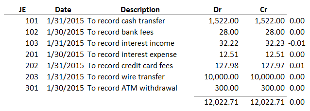
Our objective is to create an alert when a journal entry is out of balance. Since this is Excel, there are many ways to accomplish this task. In this post, we’ll customize a conditional formatting icon set to place a little red icon next to any entries that are out of balance, as shown below.

Ready? Me too…let’s get to it.

Details

The steps to create the alert shown above are:

• Compute the diff
• Apply an icon set
• Customize the rule

Let’s take them one at a time.

Compute the diff

Computing the diff is just as straightforward as it sounds. You set up a formula that computes the difference between the debit and credit amounts. The formula results are shown below for reference.

Apply an icon set

Next, we apply a standard conditional formatting rule that uses the desired icons. This is done by selecting all of the diff cells and then picking the desired icon set from the following ribbon command:

• Home > Conditional Formatting > Icon Sets

For this post, I used the icon set named 3 Traffic Lights, but there are many other fun icons to choose if preferred.

The updated worksheet is shown below for reference.

Now, it is time to customize the default conditional formatting rule.

Customize the rule

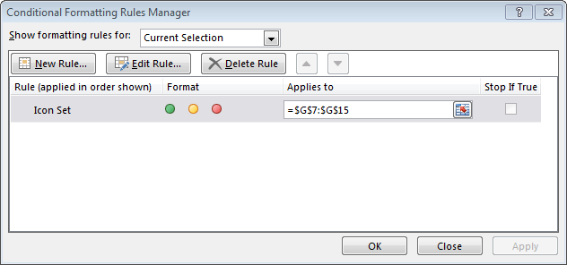
To begin, we select the conditionally formatted cells (the diff cells) and then open the Conditional Formatting Rules Manager dialog box by selecting the following ribbon command:

• Home > Conditional Formatting > Manage Rules

The dialog should look something like this:

Now, we need to edit the rule. To do so, we select the icon set rule from the list, and then click the Edit Rule button. This opens the Edit Formatting Rule dialog, as shown below.

There are many fun things to play with in this dialog, and it essentially allows us to customize the default rule settings.

By default, icon sets with three icons are applied based on the top, middle, and bottom third of the values within the range. This can be seen by inspecting the bottom half of the dialog, where we can see the green icon is used when the value is greater than or equal to 67 percent of the cell values. The yellow icon is used for those cells where the value is less than 67 percent and greater than or equal to 33 percent. The red icon is used for cells where the value is less than 33 percent. We can change these default settings.

In our case, we want to use a red icon when the cell value is greater than zero, no icon when the cell value is equal to zero, and a red icon when the cell value is less than zero. Thus, we simply update the icon, comparison, value, and type fields to the corresponding settings, shown below.

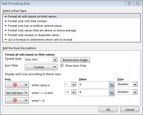
Since we don’t want to display the diff values, and we just want to see the icon, we also check the Show Icon Only checkbox, as shown above.

After applying the updates, we have achieved our goal, as shown below.

Yay…we did it!

There are many settings to play with in the conditional formatting rules manager, and I’d encourage you to check them out.

If you have any thoughts or fun conditional formatting tips…please share by posting a comment below, thanks!

Additional Resources

• Sample File
• INDIRECT function posts
• Conditional Formatting posts