Create Fiscal Year Periods with VLOOKUP

I’m a huge fan of the VLOOKUP function, and am surprised by its day-to-day utility for accountants. In this post, we use the VLOOKUP function to convert or translate calendar year transaction dates into fiscal year periods, such as a fiscal quarter. To accomplish this, we’ll first need to investigate in detail the function’s fourth argument, the range lookup argument. Let’s begin.

Range Lookup Argument

The syntax for the VLOOKUP function follows:

=VLOOKUP(lookup_value, table_array, col_index_num, [range_lookup])

Where:

• lookup_value – the value to find
• table_array – the range in which we are looking
• col_index_num – the column that has the value to return
• [range_lookup] – true or false, are we doing a range lookup?

The fourth argument, the optional range_lookup value, is the argument that enables us to easily translate dates into fiscal quarter groups, or, perform any other range lookup. So, what is a range lookup? It means we are trying to find a value between two endpoints. The word range here doesn’t refer to a worksheet range, such as A1:B10. It refers to a range between two values, such as a number between 1 and 100, 101 and 200, or in the case of dates, between 1/1/14 and 3/31/14. We are trying to find our lookup value within a range of values. Since this argument is optional, Excel users are not required to actually express a value…that is…we can leave it out of the function. The default value, if omitted, is TRUE, as in, true, we are doing a range lookup. The value of FALSE means we are not doing a range lookup, we want an exact matching value. In our case, we want to do a range lookup and so we’ll use TRUE for our formula.

Let’s give it a try.

Simple Version – Specific Year

Before we write our formula, let’s be clear about our task. We have a list of transactions. Each transaction record includes the transaction date. We need to summarize the transactions, but our company is on a 6/30 fiscal year-end. Since Excel only supports calendar year date groups, we’ll need to use the VLOOKUP function to translate the transaction dates into fiscal period groups. To prepare our worksheet, we set up a little lookup table that Excel can use to make the translation. While we are getting warmed up, we can visualize the little lookup table as follows:

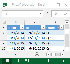
We have a from date, a to date, and a quarter label. We’ll look up the transaction date in the table to determine the quarter label.

Assuming our first transaction date was stored in cell C15 and that the little lookup table is named Table1, then the following formula would work:

=VLOOKUP(C15, Table1, 3, TRUE)

Where:

• C15 is the lookup value, the transaction date
• Table1 is the lookup range, the quarter table
• 3 is the column that has the value to return, the quarter label, which is the third column in the table
• TRUE we are doing a range lookup

The results are shown below:

The formula essentially finds the date in the lookup range and returns the quarter label.

But, we can do even better. When the VLOOKUP is finding the transaction date, it is really only looking in the first column, the “from” column, known as the lookup column. That means that it ignores the second column, the “to” column. Even though humans really love to see both date endpoints, Excel doesn’t need them. So, we can simplify our lookup table by excluding the “to” column, as shown below:

This works because the VLOOKUP function only looks for its matching value in the first column, the lookup column, and ignores other columns. After a match is found, then the function slides to the right to return a related result, in our case, the quarter label.

Quick question for you: does the quarter lookup table need to be sorted? Yes, if the fourth argument of the VLOOKUP is TRUE, then the lookup range must be sorted in ascending order by the lookup column for it to return a reliable result.

Advanced Version – All Years

We can do even better than the formula above. The lookup table above works for a specific fiscal year, but requires us to add new rows each subsequent year. Since our goal is to eliminate manual steps from recurring processes, we’ll need to figure out a way to create a lookup table that works for all years.

Fortunately, Excel provides the MONTH function which pulls the month number out of a date. By nesting the MONTH function in our VLOOKUP function, we can simplify our lookup table to include only months, as shown below.

We can use the MONTH function to pull the month out of the date, as shown below:

Remember, the lookup table needs to be sorted in ascending order for the function to return a reliable result. Since this table includes months only, it can be used for transactions that span many fiscal years.

And that my friend is my preferred method for translating transaction dates into fiscal periods. If you have other methods, please share by posting a comment below…thanks!

Additional Resources

• Sample File: FiscalPeriods
• Tables: this post relies on the table feature…if you haven’t played with it yet check out the table related blog posts