Count Distinct Values in an Excel 2013 PivotTable
This post demonstrates how to count the number of distinct (unique) values in an Excel 2013 PivotTable. Prior to Excel 2013, this capability was not built-in to the PivotTable feature. For Excel versions earlier than 2013, there are a variety of different workarounds available, some use VBA code, some use helper formulas, and some of them use functions such as COUNTIF, COUNTIFS, and SUMPRODUCT. The good news is that beginning with Excel 2013, this capability is built-in to the standard PivotTable feature. This post demonstrates how to perform a distinct count with an Excel 2013 PivotTable.
Objective
First, let’s review our objective. We have some sales transactions with region, item, and amount columns, as shown below.
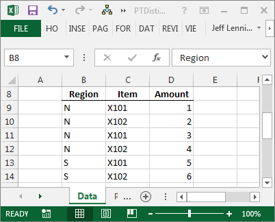
Our objective is to create a PivotTable that counts the number of unique region/item combinations. For example, we want the PivotTable to show that for region N, the count of unique items is 2.
Traditional PivotTable Limitation
With Excel 2010 and earlier, the best we could do is to count the number of transactions (rows) with any given region/item combination. This is illustrated in the screenshot below.

The count illustrated above is not what we want. We do not want to count the number of transactions/rows, we want to count the unique, or distinct, number of region/item combinations. We want a PivotTable that reports 1 for E since there is one unique region/item combination for E (X101). We expect 2 for N, since there are two items for N (X101, X102). We expect 4 for S, since there are four items (X101, X102, X103, X104). We expect 3 for W (Y200, Y201, Y202).
Excel 2013 Distinct Count PivotTable
To obtain a distinct count in an Excel 2013 PivotTable, here is what we do. We select any cell in the data source, as normal, and then click Insert > PivotTable, as normal. However, we need to add this data source to the Data Model. This is easily performed by checking the relevant check box in the Create PivotTable dialog box, as seen below. Please note, this “Add this data to the Data Model” checkbox is a new option with Excel 2013.

Next, we build the PivotTable as we normally would by inserting the region and item fields into the Rows area. Next, we insert the item field into the Values area. Now, this is the good part. We open the Values Field Settings dialog box for the item field we placed into the Values area, and look…a brand new option! The Distinct Count choice in the Summarize value field by list box, as shown below, is new in Excel 2013.

Clicking OK results in the glorious PivotTable pictured below.

As you can see, our desired counts are all here, E is 1, N is 2, S is 4 and W is 3.
If it is not important to see the item labels, we can remove the item field from the Rows area, or, hide the detail; either way is fine. This will result in the PivotTable below.

So, that is a great new PivotTable enhancement rolled out in Excel 2013. Thanks Microsoft!
Excel file used in the above screenshots: PTDistinctCount
Excel is not what it used to be.
You need the Excel Proficiency Roadmap now. Includes 6 steps for a successful journey, 3 things to avoid, and weekly Excel tips.
Want to learn Excel?
Our training programs start at $29 and will help you learn Excel quickly.
Maybe you could point me in the right direction. Your last pic shows your collapsed pivot table with a Grand Total of 7. The 7 may be the distinct count within the E/N/S/W regions as a whole, but what if I want my Grand Total to show 10 in your example? The distinct count is pretty slick, but I’d like to find a way to get my Grand Total to actually sum all of the subtotals. I haven’t found anything online addressing this particular concern.
John,
Happy to help out. To clarify this for future readers, the Grand Total 7 in the final screenshot above represents the number of unique items in the population. And, this is misleading because if we visually add up the report, we expect that to reflect a total of 10, because 1+2+4+3=10. This total represents the number of unique Region/Item combinations (rows).
So, the question is, how to update the PivotTable report to reflect the desired total of 10, rather than the default value of 7.
Since this is Excel we are talking about, there are many ways to accomplish this. Here are just a couple of ideas.
Running Total Column

One way is to modify the PivotTable report to include an additional running total column. To add the running total column, simply insert the Item field into the Values area again, and set the field to display the Distinct count. Next, change the settings to Show Values As…and select Running Total In.
The result is shown below:
Remove Duplicates
Another method is to use the Remove Duplicates feature. This takes only a few moments. Basically, copy the Region and Item columns from the source data, and paste them into a blank sheet. Then, select the range and select Data > Remove Duplicates. Confirm the dialog box, and click OK. This feature removes duplicate values, resulting in a list of unique Region/Item combinations. The resulting number of unique rows (10) is displayed in the dialog box. If you need to show the total in the report, a standard COUNTA function, or other counting function, can be used to compute the number of remaining rows.
In addition to these options above, I’d love to have some comments below if you guys would like to suggest any other approaches.
Thank you so much…. I have been looking for this for so long….
Dear Jeff,
May I know how to do it through vba?
Best regards,
Jason
Jason,
Thanks for your question about accomplishing this task with VBA. I’ll consider it for an upcoming blog post…thanks!
Thanks
Jeff
Jeff, I see your command to check the box for Add This Data To The Data Model. What does it mean when this box is grayed out, preventing me from even having the ability to check it? Thanks for any assistance!
Thomas,
Generally speaking, when the PivotTable source data is stored in an Excel worksheet, the Data Model checkbox is enabled. There are some restrictions however, such as the version of Windows and if there are multiple tables. Here are a couple of links that may be able to help determine why the Add to Data Model checkbox is disabled in your workbook, I hope they can help out:
http://blogs.office.com/2012/08/23/introduction-to-the-data-model-and-relationships-in-excel-2013/
http://office.microsoft.com/en-us/excel-help/create-a-data-model-in-excel-HA102923361.aspx
If you figure it out, I’d love a quick update comment in case others encounter a similar restriction…thanks!
Thanks
Jeff
I ran into this same issue. I noticed my workbook was open in Compatibility mode. So I closed it and reopened it and it was no longer in Compatibility mode, and the box was no longer grayed out when creating the Pivot Table. So that was the issue for me.
Thanks!
Thomas, I ran into this problem as well and resolved it promptly by making sure I was in a saved .xlsx file… initially I had been working in .csv and Excel 2013 doesn’t like letting you add the Data Model unless you’re actually working in the .xlsx file. Good luck, I hope this helps.
Scott – thank you for the comment!
Thanks
Jeff
Hi Jeff,
I found that the box was grayed out when I initially opened my file in CSV format using Excel 2013. After I saved it as an Excel Workbook (.xlsx) the “Add This Data…” checkbox was enabled. I also confirmed that the box is grayed out when the file extension is XLS (Excel 97-2003 Workbook) instead of XLSX.
Thanks for posting this procedure; it came in quite handy for me recently!
Jeff
Jeff,
I appreciate you taking the time to post the information about the impact of the file format…thanks!
Thanks
Jeff
I have just began using this distinct count and already have an issue with it counting blank cells as 1. I have researched online and others have posted the same issue but I have not seen a solution. Any ideas?
Thanks
Mike
Hey Mike,
For a Pivot Table to work properly, the data can’t contain any blank cells. That little tip should help your situation:)
Let me know if I can be of more help,
Kurt LeBlanc
Thank you so much sir……
Hi Jeff,
It is also greyed out when I use external data source via ODBC. I did not find a way to work around this. Any ideas?
BR Per
Hi Per
I found this reply from Mr. Jeff to another student:
Generally speaking, when the PivotTable source data is stored in an Excel worksheet, the Data Model checkbox is enabled. There are some restrictions however, such as the version of Windows and if there are multiple tables. Here are a couple of links that may be able to help determine why the Add to Data Model checkbox is disabled in your workbook, I hope they can help out:
http://blogs.office.com/2012/08/23/introduction-to-the-data-model-and-relationships-in-excel-2013/
http://office.microsoft.com/en-us/excel-help/create-a-data-model-in-excel-HA102923361.aspx
If you figure it out, I’d love a quick update comment in case others encounter a similar restriction…thanks!
Kurt LeBlanc
thanks!!!
thankyou so much .It was a grt help.
Dear Jeff
Thankyou so much – well explained and has helped me with an excel problem that I had been struggling to fix – until now.
Cheers
Rod
Hi everytime I refresh my pivot, the pivot table disappears.
Can you please advise
I’ve also been trying to find a resolution to this problem!
I recently started using this to show a number of claims rather than number of lines on the sheet. Problem is I update the data weekly and now when I go to refresh it doesn’t let me change the source to the new spreadsheet I will be pulling the data from.
Distinct Count is not appearing in pivot table of Off 2016 – any one have seen this option in value field settings..