Count and Sum Negative Numbers

Welcome to our tutorial on how to count and sum negative numbers in Excel! We will cover three exercises where we will learn how to utilize COUNTIF, SUMIF, and conditional formatting to count, sum, and identify negative transactions. By the end, you will have multiple techniques to operate on negative numbers in Excel. Let’s jump right in!

Video

Walkthrough

Let’s work through this one exercise at a time.

Exercise 1: Counting Sales Transactions and Returns

Let’s start by counting the number of sales transactions (positive amounts) and returns (negative amounts) with the COUNTIF function.

Consider our transaction list:

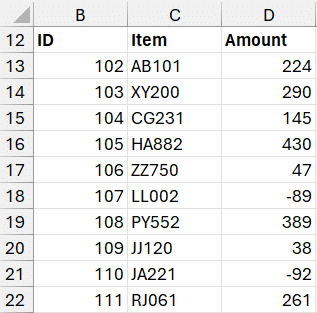
Take note of the transactions, where positive numbers represent sales and negative numbers represent returns.

To count sales transactions (positive number), we use the following COUNTIF formula in C7:

=COUNTIF(D13:D22,">=0")

• D13:D22 is the range of cells to count
• “>=0” is the criteria, greater than or equal to 0 enclosed in quotes.
• Note: you could also use “>0” if you wanted to exclude any 0 dollar transactions from the count

We can similarly count the returns (negative number) with the following formula in C8:

=COUNTIF(D13:D22,"<0")

• D13:D22
• “<0” less than 0 enclosed in quotes
• Note: you could also use “<=0” if you wanted to include 0 dollar transactions in the count

The results are below:

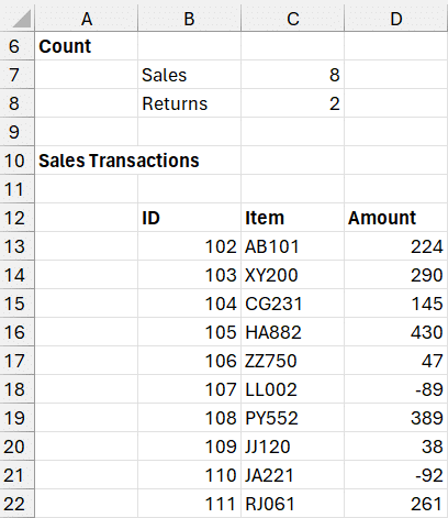
As you can see, there are 8 positive cells (sales) and 2 negative cells (returns) in the range.

Rather than counting the cells, let’s say we want to sum the amounts. Let’s tackle that in the next exercise.

Exercise 2: Summing Sales Transactions and Returns

In this exercise, we’ll calculate the sum of the sales transactions and returns using the SUMIF function.

Same basic transactions as the previous exercise.

This time, we use the SUMIF function instead of COUNTIF.

For the sales transactions (positive), we use the following in C7:

=SUMIF(D13:D22,">=0")

For the returns (negative), we use the following in C8:

=SUMIF(D13:D22,"<0")

The results are shown below:

Excellent! Now, what if instead of counting or summing the values, we just wanted to identify the negative values. Well, for that we can use conditional formatting … let’s tackle that next.

Exercise 3: Identifying Negative Transactions Using Conditional Formatting

Let’s say that instead of counting or summing, we wanted to simply identify the negative transactions. Depending on what you are working on, probably the fastest way to identify negative values is to simply change the sort order. Alternatively, you could apply a filter. But, depending on what you are working on, you may want to apply some type of cell format to the negative numbers. This is when we can turn to conditional formatting.

We will talk about two options: first, we’ll format the Amount cells ONLY. Then, we’ll format the entire transaction (all data columns).

To highlight the Amount cells only, select the amount cells. Then, use Home > Conditional Formatting > Highlight Cell Values > Less Than and enter 0. Hit OK and bam:

Now, let’s highlight the entire transaction rather than just the amount.

First, select the entire transaction range, and make a note of the one Active Cell within the selected range. Note: this is typically the upper left cell.

Home > Conditional Formatting > New Rule. In the resulting New Formatting Rule dialog, select “Use a formula to determine which cells to format.”

Then we can use a simple comparison formula, where you lock in the column reference of the active cell and use a relative row reference. So, assuming the active cell is D9, you would use this:

=$D9<0

Then, click the Format button and pick your desired format:

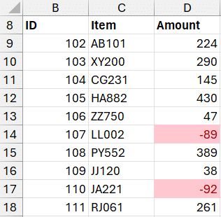
Once we hit OK to apply the conditional formatting rule, bam:

And now we have highlighted the negative transactions!

Conclusion

I hope this tutorial has provided three three useful techniques to operate on negative numbers. We learned how to use COUNTIF and SUMIF functions to calculate the count and sum of positive or negative transactions. We applied conditional formatting to identify negative transactions without affecting the original sort order. If you have any suggestions, questions, alternatives, or improvements, please post a comment … thanks!

Sample file

FAQ:

Q: Can I use these techniques for counting positive numbers as well?

Absolutely! By adjusting the criteria in the COUNTIF and SUMIF functions, you can count or sum positive numbers easily.

Q: What if I want to count or sum numbers within a specific range?

You can specify a range in the COUNTIF and SUMIF functions by modifying the cell range argument as desired.

Q: Can I combine multiple criteria in the COUNTIF and SUMIF functions?

Although COUNTIF and SUMIF are designed to operate on a single condition, COUNTIFS and SUMIFS are designed to operate with multiple conditions.

Q: Is it possible to change the format or appearance of the cells using conditional formatting?

Yes, you can choose various formatting styles, colors, and even highlight cells based on specific conditions using conditional formatting.