Battle of Heavyweights: Round 5

Round 5 begins now! In this post, the goal is to understand the results of each function when no matching rows are found. That is, when the lookup value is not found in the data table. Do the functions return an error? The closest match? 0? Well, that is why we are here, so let’s find out.

Round 5

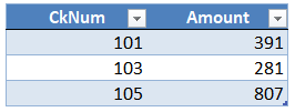
Let’s say we are trying to do a bank reconciliation. To do this, we start by getting a list of checks from our check register:

Next, we grab a list of checks that have cleared the bank (Table1):

Our goal is to write a formula to retrieve the amount of the checks that have cleared the bank.

Let’s try them one at a time, starting with VLOOKUP.

VLOOKUP

We start with VLOOKUP (TRUE), and write the following formula into C8:

=VLOOKUP(B8, Table1, 2, TRUE)

We fill the formula down, and hmmm:

Even though check 102 does NOT appear in the bank list (Table1), the formula returns 391, which is the same value as check 101. Why is this? It is because we instructed VLOOKUP to perform a range lookup when we used TRUE for the 4th argument. This was discussed in a previous post. So, when we use VLOOKUP TRUE, it returns a result by performing a range lookup.

Since this isn’t what we want here, we’ll use FALSE to tell VLOOKUP to perform an exact match. We update our formula as follows:

=VLOOKUP(B8, Table1, 2, FALSE)

And fill the updated version down:

Interesting. It returns #N/A when no matching value is found. This let’s us know that the check number is not found in the bank activity, which is good. But, what is also interesting is that the Total formula also returns #N/A. Why? Because any formulas that depend on the range inherit the error … meaning … the error trickles down to any other formulas that reference cells with the error.

So, VLOOKUP FALSE returns #N/A when no matching values are found.

Now, what about SUMIFS?

SUMIFS

We write the following formula into D8:

=SUMIFS(Table1[Amount],Table1[CkNum],B8)

And fill the formula down:

Interesting! SUMIFS returns 0 when no matching rows are found. This means that the Total formula works, and any other formulas that depend on the range work.

So, SUMIFS returns 0 when no matches are found.

Analysis

So, let’s recap what we discovered in this round:

When no matching rows are found, VLOOKUP TRUE perform a range lookup, VLOOKUP FALSE returns #N/A, and SUMIFS returns 0

So, who wins the round? Well, let’s ask ourselves the question … in practice, which function would we use? The answer is really: it depends.

It depends on what we are working on. For example, if we are performing a list comparison, and want to know for sure that a value does or does not appear on the related list, we need to use VLOOKUP FALSE. We can’t rely on the results of SUMIFS because it would return 0 when the item is not found AND if the sum of all matching rows is 0 (for example, if you add a row with 100 to another row with -100, the net is 0). We can’t distinguish between these two results.

But, if we aren’t performing a list comparison, and want to avoid an error trickling down throughout dependent formulas, we could use SUMIFS.

So, once again, who won? I’d have to say it is a draw. It really just depends on the workbook.

So, both receive 10 pts!

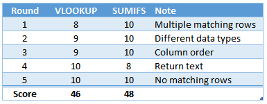
Updated scoreboard …

Updated stats …

Alright, we’ll see you in the next round!

Note: we could use IFERROR with VLOOKUP to replace #N/A with 0 like this: =IFERROR(VLOOKUP(…),0)

Sample file: Round5.xlsx