PPMT Explained: Dynamic Loan Schedule

Managing loans and tracking monthly payments just got a whole lot easier. In this tutorial, we’ll explore the PPMT function in Excel—a lesser-known but incredibly powerful function that calculates the principal portion of a loan payment for a specific period. Even better, we’ll show how to transform this function into a fully dynamic loan amortization schedule. Whether we’re dealing with a 3-month or a 60-month loan, everything updates automatically.

Video

Step-by-Step Guide

Let’s take this step-by-step and build a professional, interactive schedule using built-in Excel functions like PPMT, PMT, and SEQUENCE. If you’re ready for a practical, educational dive into making Excel work smarter for you, let’s jump in!

Step 1: Set Up the Loan Terms

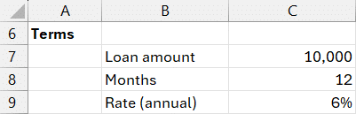
To start, we’ll need a set of inputs that define the basic loan terms. In a clean Excel sheet, enter the following values in your worksheet:

• Loan Amount: 10,000 (cell C7)
• Number of Months: 12 (cell C8)
• Annual Interest Rate: 6% (cell C9)

Step 2: Calculate the Monthly Payment

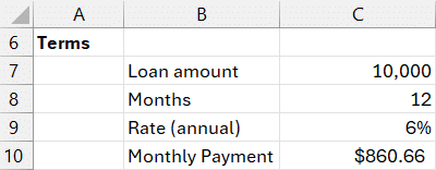
We’ll use the PMT function to find the regular monthly payment amount. Enter this formula in cell C10:

=PMT(C9/12, C8, C7)

Explanation:

• C9/12: Converts the annual rate to a monthly rate
• C8: Number of periods (months)
• C7: The loan amount (present value)

This gives us the monthly payment.

But how much of each payment goes toward principal? Let’s dig deeper.

Step 3: Calculate Principal Payment Using PPMT (Single Month)

To find the portion of a payment that applies to principal for a specific month, we use the PPMT function:

=PPMT(C9/12, 1, C8, C7)

This returns the amount of the monthly payment that is applied to principal reduction for month 1 (after interest). To make this formula more flexible (allowing us to more easily check other months without having to update the formula arguments manually), we can use a cell reference instead of the hardcoded 1. For instance, if the month number we want to check is stored in B15, update the formula as:

=PPMT(C9/12, B15, C8, C7)

This way, we can change the value in cell B15 to any month and instantly see what portion goes to principal for that month. Now that we have the basics, let’s scale this up into a full schedule.

Step 4: Create a Dynamic Loan Amortization Schedule

Now, let’s build a complete loan amortization schedule using dynamic arrays (no drag-down formulas).

Generate Month Numbers with SEQUENCE

In cell B15, enter the following:

=SEQUENCE(C8)

This creates an array that lists numbers from 1 to the number of months in the loan in C8 (e.g., 1-12 for a 12-month loan).

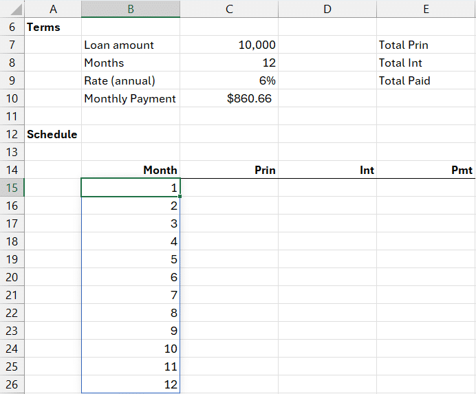
It’s dynamic and updates automatically if we change the number of months.

Calculate Monthly Principal Payments

In cell C15, next to the generated month numbers, enter:

=PPMT(C9/12, B15#, C8, -C7)

We used the spill operator (#) to apply the formula across all values in B15. This outputs a dynamic array listing principal payments for each month.

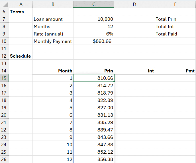
No dragging formulas required!

Calculate Monthly Interest Payments

We already calculated the monthly payment amount in cell C10. To get the interest portion for each month, one approach is to subtract the principal payment from the total payment. Enter into D15:

=C10 - C15#

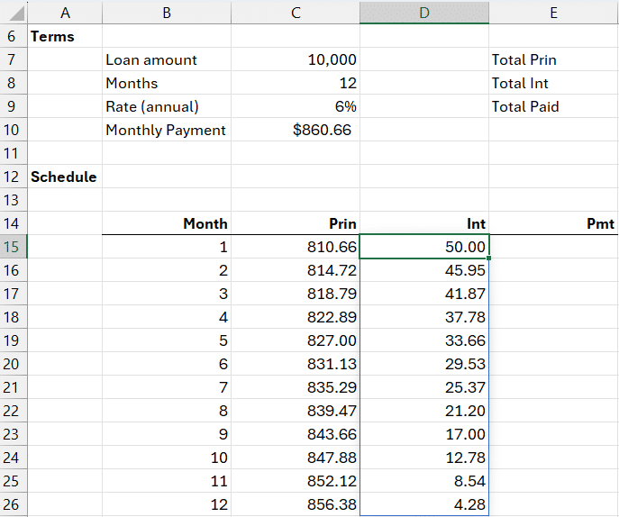
This uses array behavior to subtract the entire principal range from the monthly payment, leaving us with the interest portion.

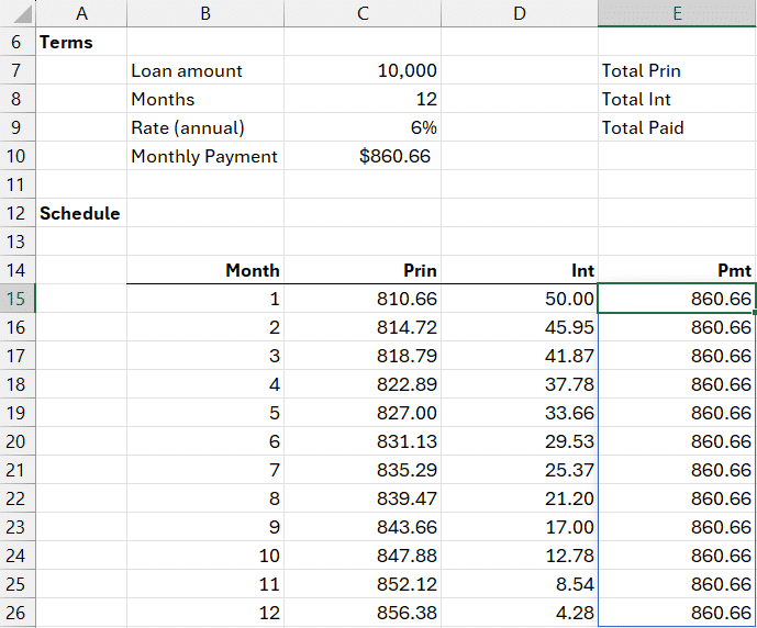
Verify Total Payments

Let’s confirm the math adds up. In cell E15, enter:

=C15# + D15#

This should match our total monthly payment from C11 for each row.

Step 5: Summarize the Loan Payments

Let’s wrap the schedule with a few key totals at the top of the schedule:

• Total Principal: in F7
  =SUM(C15#)
• Total Interest: in F8
  =SUM(D15#)
• Total Paid: in F9
  =SUM(E15#)

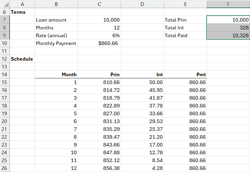
These totals adjust dynamically based on the loan terms. Want a 24-month loan? Change the value in C8, and your entire schedule updates instantly.

Note: Flip the Signs

Since Excel’s financial functions treat borrowed money as a cash inflow (positive), results may appear as negative values. If we prefer positive numbers, we can easily fix this with a leading – before our function:

=-PPMT(...) and -PMT(...)

Summary

With a combination of PPMT, PMT, and SEQUENCE, we’ve built a fully functional and self-updating loan amortization schedule that adjusts based on loan amount, rate, and duration. No need for manual copying or helper columns—just clean, dynamic Excel solutions. This is a fantastic tool for anyone working on financial modeling, small business planning, or personal budgeting.

Download the Excel File

Frequently Asked Questions

What is the PPMT function in Excel used for?

The PPMT function calculates the principal portion of a payment for a given period of a loan.

What’s the difference between PPMT and PMT functions?

PMT gives the total monthly payment (principal + interest), while PPMT gives only the principal payment for a specific period.

How do I calculate the interest portion of a payment?

Either use the IPMT function or subtract the principal payment (PPMT) from the total payment (PMT) to get the interest portion.

How can I make the loan schedule dynamic in Excel?

Use the SEQUENCE function to generate period numbers and apply array formulas with the spill operator (#).

Why is the result coming in negative?

Excel financial functions use cash flow logic: money paid out appears negative.

Can I use this for different loan durations?

Yes! The schedule adjusts dynamically based on the value entered in the “Number of Months” cell.

Does this method require copying formulas down?

No. Because we use dynamic arrays and the spill operator, Excel handles multiple rows automatically.

Is this method available in all Excel versions?

Dynamic arrays like SEQUENCE and spill behavior are available in Excel 365 and Excel 2019+. Older versions may require helper columns.

Can I add extra payments or adjustments?

Advanced customizations like extra payments can be added with more formulas, but this tutorial focuses on standard amortization.

Why use SEQUENCE instead of manually numbering rows?

SEQUENCE auto-generates rows based on inputs, making the schedule fully dynamic and easier to maintain.