Impossible PivotTables 1 – Calculated Fields

This is the first post in a series called Impossible PivotTables. The purpose of this series is to explore Power Pivot. I thought a fun way to do that would be to demonstrate how using the data model enables us to build PivotTables that are either impossible with traditional PivotTables or that require workarounds. I hope it provides an enjoyable way to examine Power Pivot 🙂

Impossible PivotTables?

Historically, when I tried to build a traditional PivotTable (PT) that wasn’t supported by Excel, I’d have to figure out some type of workaround. These workarounds weren’t always pretty, but, they helped me get the numbers I needed. I’d use workarounds like adding helper columns to the data table, copy/pasting multiple data tables into a single data source table, clicking-and-dragging to manually sort the labels, or creating formulas outside the PT on the worksheet. All of these worked, sort-of, but, they didn’t feel very elegant. They didn’t feel very reliable either … they felt fragile, like they could easily break in future periods when I had to update the report. Then, everything changed when I learned about Power Pivot (PP).

Power Pivot essentially allows us to combine the mathematical ability of formula-based reports with the PivotTable feature. It allows us to build PT reports that don’t require the workarounds mentioned above. The result is a clean, reliable report that is easy to update and maintain over time. And, honestly, they just feel better.

So, enough background jibber-jabber, let’s go build our first impossible PivotTable.

Objective

Traditional PivotTables are great at summarizing and aggregating values that are stored within a data source table. When you need your report to compute values that aren’t included within the data source, you can create Calculated Fields. However, this feature is not very robust and has limitations. For example, a calculated field can operate on values within the report, but not on values outside of the report in another range or table. So, when we encounter this limitation, we try to work around it. For example, we may add a helper column to the data table or decide to perform the calculations outside of the PT. But, these workarounds have issues. For example, adding a helper column in the data table may not provide the desired math in a given report. That is, the math may need to operate on aggregated subtotals or totals rather than on each row. And when we create formulas outside of the PT, they aren’t refreshed along with the PT … meaning we need to babysit them to be sure they are filled down for new rows.

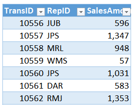
To illustrate this issue, I’ll provide an example report that computes commission based on sales data. Let’s say we have a bunch of sales transactions, as shown below.

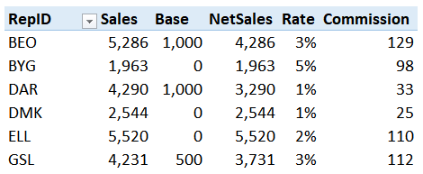
Then, we have each of the rep’s commission rates and base values in another table, as shown below.

The report we’d like to create will add up the sales transactions, subtract the base sales amount, and then multiply the resulting net sales amount by the corresponding commission rate. We are after something like this:

Before we even start building the report with a traditional PT, we encounter a problem. A traditional PT supports a single source data table, but our data comes in two tables. But, let’s set that fact aside for the moment and focus on what we can do. We can easily use a traditional PT to summarize the sales by rep, so we start with that. We create the PT and insert the RepID and Sales fields.

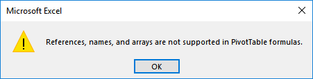
Next, we try to create a Calculated Field to compute the commission values. The formula would basically use VLOOKUP to retrieve the commission rate and base amount for each rep. We open the Calculated Field dialog and when we enter a formula that tries to reference values outside of the PT, such as the commission rates table, we receive the following error message:

So, we quickly conclude this is an impossible PivotTable and try to come up with a clever workaround. For example, we try using a helper column in the data table to retrieve the commission rates. And that works, but when we go to compute the commission amounts, we realize that we need to aggregate the sales values and subtract the base before applying the rate. So, we hit a dead-end with that and try something else.

We proceed to compute commission outside of the PT in normal Excel cells. When we do this, the final report isn’t even a PT … it is a formula-based report that references an intermediate PT for the aggregated sales values. And while it provides the numbers we need for this month, what about next month? When we think ahead, we realize that this approach is fragile and may break next period when we update the report. When formulas are written outside the PT, they won’t be included when the PT is refreshed. So, hopefully we’ll remember to fill the formulas down manually to include any new reps. And, as you may imagine, this is where Power Pivot comes in to help us out.

This PivotTable is possible when we use Power Pivot instead of a traditional PivotTable… and no workarounds are needed 🙂

Overview

We’ll build this PivotTable using the following steps:

• Load the tables into the data model
• Build the basic PivotTable
• Write the measures

Let’s get to it.

Note: The steps below are presented with Excel for Windows 2016. If you are using a different version of Excel, please note that the features presented may not be available or you may need to download and install the Power Pivot Add-in.

Load the tables into the data model

First up, we need to load the tables into the data model and relate them. To do this, we select any cell in our commission rates table and click the Power Pivot > Add to Data Model command.

We do it again for the table that stores the sales transactions. Select any cell in the data table and click the Power Pivot > Add to Data Model command.

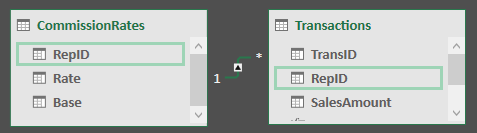
My favorite way to relate these two tables is by using diagram view, so, inside the Power Pivot window, we click Home > Diagram View. We can see the two tables, as shown below.

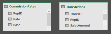
Next, we need to tell Excel how these tables are related to each other, that is, which column is shared between them. In our case, it is the RepID column. So, we click-and-drag the RepID from one table to the other. Excel adds the relationship line, as shown below.

With this complete, it is time to build our basic PT.

Build the basic PivotTable

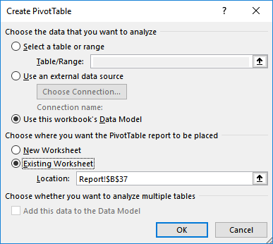
To get our PivotTable started, we use Excel’s Insert > PivotTable command. In the resulting dialog, we want to Use this workbook’s Data Model, as shown below.

Next, we insert the CommissionRates[RepID] field into the Rows area, and the Transactions[SalesAmount] and CommissionRates[Base] fields into the Values area. The basic report is shown below.

With our basic PT looking good, it is time to do the remaining calculations by writing a couple measures.

Write the measures

First, we need to subtract the base sales from the sum of sales to determine the commissionable net sales amount. To do this, we use the Power Pivot > Measures > New Measure command. In the resulting dialog, we enter the desired measure name, NetSales, and the corresponding formula as shown below.

Then, we repeat the steps to create our next measure, Commission, which multiplies the NetSales measure by the commission rate, as shown below.

We can toss the NetSales measure, the Rate field, and the Commission measure into the values area of the PivotTable, and the updated report is shown below.

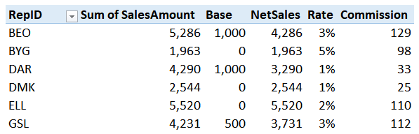
And look … no workarounds in sight. It is like Power Pivot made an impossible PivotTable possible 🙂

If you’d like to investigate the details, please check out the sample file below. And if you have any other fun Power Pivot tips, please share by posting a comment below.

Sample File

• Commission2.xlsx