How to Return a Value Left of VLOOKUP’s Lookup Column
If you have ever tried to return a value that physically lies to the left of the lookup column, you quickly realize that this task is difficult to accomplish with the VLOOKUP function. This is a perfect time to move beyond the VLOOKUP function and explore the INDEX and MATCH functions.
Note: depending on your version of Excel, you may have XLOOKUP as an option … more info here: https://www.excel-university.com/xlookup/
Overview
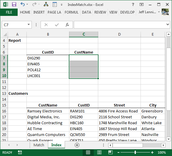
Consider the following screenshot.
We are trying to populate the report’s CustName column. We would like to look up the CustID from the Customers table, and return the CustName. The problem is that in the lookup range, the CustName column lies to the left of the CustID column. That is, the return column lies to the left of the lookup column. VLOOKUP is a righty, can’t go left.*
And this brings us to the reason we are here, to get the hang of using the INDEX/MATCH combination to return values that lie to the left of the lookup column. But wait, there’s more. In addition to being able to return values to the left, this combination doesn’t suffer from another common limitation of the VLOOKUP function. When the third argument of VLOOKUP is expressed as a static integer value, such as 3, a column inserted between the lookup column and the return column will break the function. Since the third argument is expressed as an integer, it will not adapt to column inserts when inserted between the lookup and return columns. The INDEX/MATCH combination does not suffer from this limitation. Since the arguments are range references, Excel adjusts the formulas to accommodate column inserts. Alright, enough talk, let’s get to it.
MATCH
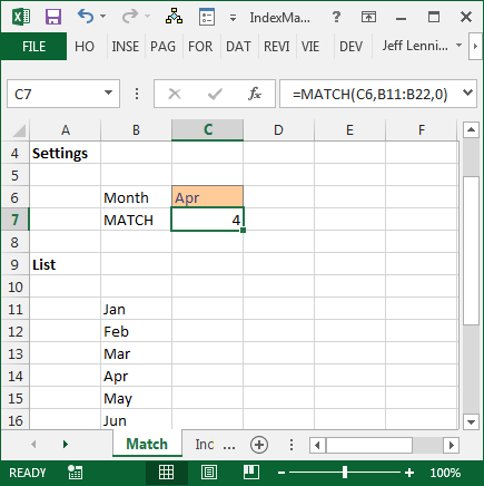
Let’s take them one at a time. The MATCH function returns the relative position of a list item. If we asked Excel to MATCH “Jun” in a list of month abbreviations, it would return 6. “Apr” would return 4. This idea is illustrated in the screenshot below.
The syntax of the MATCH function follows:
=MATCH(lookup_value,lookup_array,[match_type])
Where:
- lookup_value is the value we are trying to find
- lookup_array is where we are looking
- [match_type] is typically 0 for exact match, but there are other choices to explore here
In our screenshot, we use the following function to return the relative position of the month name:
=MATCH(C6,B11:B22,0)
We are trying to find the relative position of our month (C6), in the list of month abbreviations (B11:B22), and zero for exact match.
Just remember, the MATCH function returns the relative position of a list item.
INDEX
The INDEX function returns the cell value from a range at a given position. Technically, it does much more than that, but since we are just getting warmed up, let’s stick with that idea: it returns a cell value from a list at a given position.
The syntax of the INDEX function follows:
=INDEX(array, row_num, [column_num])
Where:
- array is the range that has the value you want to return
- row_num is the relative row position that has the value you want to return
- [column_num] is the optional column number, useful when performing two-dimensional lookups
What we’ll do is use the INDEX function to return a cell value, and we’ll nest the MATCH function in there so that it can tell the INDEX function which row has the value we want. Our INDEX/MATCH formula will look something like this:
=INDEX(array, MATCH(...))
Where the MATCH function figures out the row number argument. The MATCH function returns the relative row number to the INDEX function.
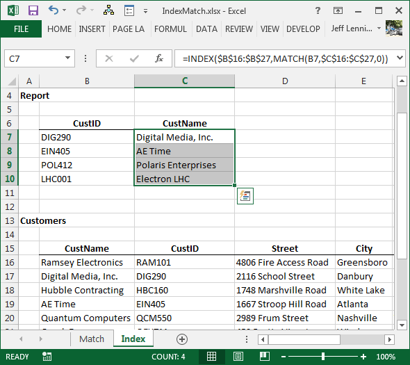
Consider the screenshot below:
We used the INDEX function to return a value from the CustName column. For the row_num argument, we used the MATCH function to determine the relative position of the CustID within the CustID column.**
The formula used in C7 is:
=INDEX($B$16:$B$27,MATCH(B7,$C$16:$C$27,0))
Where:
- $B$16:$B$27 is the list that contains the value we wish to return, the CustName column
- MATCH(B7,$C$16:$C$27,0) determines the row for the INDEX function
- Where:
- B7 is the value we are trying to find, our CustID
- $C$16:$C$27 is where we are looking, the CustID column
- 0 means exact match
The INDEX/MATCH combination is quite handy, and can be used to return values that lie to the left of the lookup column.
If you want to play with these functions a bit, feel free to download the IndexMatch Excel file that was used to prepare the screenshots for this post:
Notes
* There is a very creative way to have the VLOOKUP function go left, which is to use the CHOOSE function as the second argument. Wow, when I read Richard Schollar’s post on Bill Jelen’s site, I was so impressed! Well done!
** The thing that can be often confusing for long-time VLOOKUPers is the order of the arguments. VLOOKUP begins with the value we are trying to find. We think about the VLOOKUP function like this: go find this, comma, in here, comma, return this. When using the INDEX/MATCH combination, the thinking reverses. We first specify the column that has the value we wish to return. The thinking becomes this: from this column, return this value.
Excel is not what it used to be.
You need the Excel Proficiency Roadmap now. Includes 6 steps for a successful journey, 3 things to avoid, and weekly Excel tips.
Want to learn Excel?
Our training programs start at $29 and will help you learn Excel quickly.


Bundle of thanks……..
Thank you very much.
I was looking for this from many day.
can I like this comment? same here!
Wow! Thanks a million. This help me so much and your explanation was simple enough that I understood what I was doing. Thanks again!
Wow…. was looking for this from long time. This is great information. Thank you so much. Please share if you have advance excel details
That is a fantastic skill!!!!!! Millions of thanks it saves me so many works on Excel and even VBA!!!
THANK YOU VERY MUCH!!!!!!!!!!!!!!!!!!!!!
Thanks. I was looking for this excel ‘trick’ for getting help in my data nalsyis.
Hi all
I have been using =IFERROR(INDEX($F$13:$F$1353, MATCH(0,COUNTIF($X$12:X12, $F$13:$F$1353), 0)),””) and it work perfectly in order to bring unique values from a column with repeated values. However I use a filter on the repeated values column “F” and when I deselect any item from the “F” filtered column I would like to have this item removed from the unique items list created. Couldn’t figure out a formula to make this work.
Thanks in advance!
Hey Lucas
I don’t know of any formula to help you accomplish that…but I do know a Query can be set up to do this and all you do is refresh it:)
Let me know if you need help setting that up,
Kurt LeBlanc
Thanks a lot!!.. Really helpful 🙂
why excel cannot develop vlookup-left function? same as hlookup-up? same format of functions, right?
Yang,
The INDEX() function in Excel can go left as you pointed out. It returns a value given the intersection. I recommend using MATCH() with it to make the formula versatile.
Thanks,
Kurt
good…
Nicly explained
Genius…well explained , you saved my time, Thank you very much…
Wonderfully explained and has saved me so much time. Thank you very much!
Well done! One of the clearest and most concise articles on Excel I have seen.
Thanks Kevin!
thanx, helped me solve my back column vlookup issue.
🙂
Brilliant !! Thank you so much for saving me lots of frustrating hours trying t solve this “leftie-vlookup” thing!
🙂
Thank you for explaining how to think in “notes **”. That made it all clear to me!
Great solution. Simple, concise, effective. Many Thanks to you
Thank you so much!!!
For those who like to do this via a custom VBA UDF function (as that’s also easier to explain to non-Excel guru’s):
Function rev_vlookup(searchString As Variant, searchRange As Range, resultsRange As Range, Optional columnIndexInResultsRange As Integer = 1, Optional exactMatch As Boolean = False)
rev_vlookup = Application.WorksheetFunction.Index(resultsRange, Application.WorksheetFunction.Match(searchString, searchRange, exactMatch), columnIndexInResultsRange)
End Function
Very cool…thanks for sharing!!
How can I get it to return a list of matches beyond the first one it finds. I need it to return several matchs
Hi Al,
I believe you are looking for SUMIFS(), AVERAGEIFS(), COUNTIFS()…They give you the result of every row that matches your criteria:) If you need further help, I’m happy to assist in any way I can!
Kurt LeBlanc
Thanks a lot for this, Jeff. Much appreciated.
I have this working. Now the only thing is, if the text doesn’t have a match it returns #N/A. I would like it to return a 0 when there isn’t a match. How do I do that?
Thank you.
You could wrap the IFERROR function around it, like this =IFERROR(INDEX(…),0)
Thanks
Jeff
Thanks u sir!
Thank u so much sir….you explained it in a very simple way..
thanks good
Thanks you So much. It is working great.
Very good:)
Kurt LeBlanc
I need to set up a list of race practice times from fastest to slowest, reading values from a master sheet completed by the runner. There is only one practice time for each day. I have a list of times from fastest to slowest (SMALL fn). I’ve then used VLOOKUP and INDEX/MATCH to find that time (eg. fastest, 2nd fastest) on the master sheet and return the date for that race time. However, where two or more race times are the same, the same date is returned all, even though all 2 or 3 races were run on different days. I get the same outcome with both VLOOKUP and INDEX/MATCH. How can I display the unique date relating to each race time (ie. the date that is in the same row as the race time)? Grateful for any advice you can provide.
Hey Soysoi
I’m not sure if I am reading this correctly, but have you tried just sorting the data by race time and date? You can apply a custom sort and sort by time and ,within each time, by date, so it gives you the earliest date first when you run the same times.
Let me know if that helps or if I can help you further:)
Kurt LeBlanc
What If I have repeated values to be lookup for. Example what if Ramsey Electronics and Digital Media, Inc has the same cust ID, it will return only 1 value. How to go about it?
If the value you are trying to return is numeric, like the sum of multiple amounts, then you can accomplish that with SUMIFS instead of VLOOKUP. More info on that here: https://www.excel-university.com/multiple-condition-summing-in-excel-with-sumifs/
Very Very Thanks…………….
Welcome 🙂
thanks, saves a lot of time!!
To the million thanks you have received already, let me add a zillion or two. A brilliant explanation of a very complex set of functions. It all worked first time for me and I learnt a lot in the process. Thanks very much.
Welcome Mike…glad to help 🙂
love this formula
Me too 🙂
Thank you this information of Return value v lookup
HI All
I am looking for a solution to the probles as:
I have custId and date as one column say in table 1 and in table 2 i have corresponding credit line to this column,for ex:
TABLE 1
Cust_id
AP-11-2016(AP is customer identification and 11-2016 is NOV’2016)
Now in table 2 we have credit limit column correspoding to the Cust_d ,for ex:
Cust_id Credit_limit
AP-11-2016 10,000
AP-02-2017 20,000
Now for example there is no entry for the month of (Jan’2017) in table 2 however this cust_id will be present in table 1 and we want to have that entry same credit line as of the previos month.
How do I achieve that?
I tried the “Choose” trick on a couple of hundred lines but it is REALLY resource intensive, seems it is only useful if you have information in a couple of lines only.
Thanks!!
Most Helpful Example for Index and Match, Thank You,
Thanks a lot for this post! Explained in a clear way. I already lost hours, figuring out why LOOKUP wouldn’t return my value. It did give me one, a random one. I even reinstalled excel. Only to find out LOOKUP / VLOOKUP doesn’t go to the left. Darn.
This does exactly what I’ve been looking to do for the longest time! Thank you so much for posting it, and in a way that made it super easy to use!
Welcome 🙂
I have a an excel tabulation of where i need to establish a formula for a personeel where rate is available in another tabulation but satisfying a nationality and position, can you please assist.
I would suggest using slicers for that…more info here:
https://www.excel-university.com/slicers-as-an-alternative-to-conditional-drop-downs/
Hope it helps,
Jeff
I like the INDEX function, but I always solved this issue using OFFSET, now I have another tool.
Thanks
This was super helpful for a difficult to search subject in Excel, thank you!
Welcome 🙂
Exactly what I was looking for, thank you for the very clear explanation.
Thank you very much for your assistance. Actually this is great fully assisted.
Great; I were wondering how to get this; Highly appreciate.
Question: Now that I have mastered the index/ match function may I use this to perform a bank reconciliation instead of v look up? Thanks for the help!
Yes, absolutely 🙂
Thank you!
Amazing! Thank you so much for sharing. Took a few attempts to get it right, but after reading the explanation and break down of the formula, I got there in the end.
Excellent! Thanks so much for the help!
Google Sheets make this easy:
=VLOOKUP( search_for, Query(in_range, “select D,C”), 2, False)
… or to find the nearest match if the search column is not sorted:
=VLookup( search_for, Query(in_range, “select D,C order by D”), 2, True)