How to Highlight Duplicates in Excel

A duplicate value is a value that shows up more than once in a spreadsheet. These pop up all the time when working with datasets, and they can be tedious to sort through if you don’t know the quick ways to find them. Learn how to highlight duplicates in Excel to make the process take less than a minute!

You can even customize your settings to include only the second or third time the data appears, or highlight only specific types of duplicates. There are several ways to get the job done – we’ll use the same table in each example to keep things simple.

1. Highlight duplicates in a range of cells

One easy way to highlight duplicates in Excel is to use conditional formatting. Here’s how to do it:

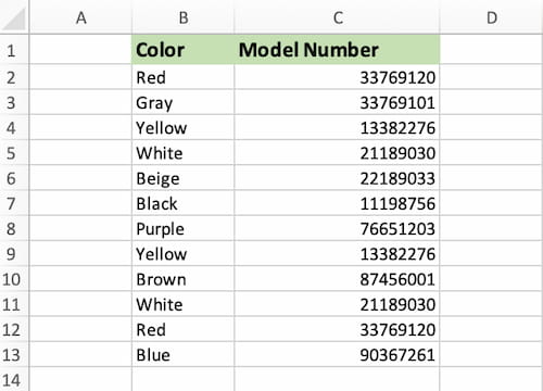
• Enter your values and select the range where you want to find the duplicates. In this example, the range is C2:C13.

Note: You can download this sample file to save some time instead of typing in all the values manually:

• Navigate over to the Home Ribbon item and select Conditional Formatting.
• Select Highlight Cells Rules and choose to highlight duplicate values. You can use several colors to highlight the cell, the text, or both.
• The final result will look like this:

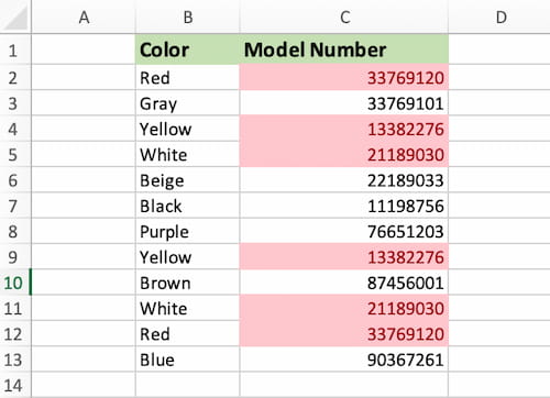
If you want to continue highlighting duplicates in your Excel spreadsheet as the list grows, just select column C and follow the same steps!

2. Highlight All Duplicate Values Except One

Let’s say you need to delete all duplicates from a spreadsheet but want to keep all unique values. If it has a lot of duplicates, it would still require you to manually sift through all the highlights to figure out which ones to get rid of.

By highlighting all duplicate values in Excel except for one, you’ll be able to easily see which ones can be kept and which ones can be eliminated.

• Start by using Sort & Filter to order column B alphabetically. This just makes it easier to compare the values.
• Select column B.
• Select Conditional Formatting and Highlight Cells Rules.
• From the drop-down menu, choose Use a formula to determine which cells to format.
• Insert the following formula: =COUNTIF($B$2:$B2,$B2)>1
• Choose your highlight color and click OK.

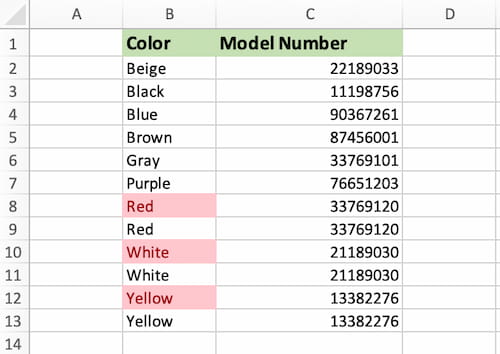
And that’s it! 

The COUNTIF function is used to count the number of cells that meet a certain criteria. In this case, the criteria is that the number of times a value is referenced is greater than 1 (seen as >1 in the above formula). 

You can use nearly the same formula to highlight data that only appears a second time:

 =COUNTIF($B$2:$B2,$B2)=2

 =COUNTIF($B$2:$B2,$B2)=3 can be used to highlight data that appears a third time, and so on.

3. Check multiple columns for duplicates

If you have a table with two columns or more and want to check for duplicates in the rows, the first two methods won’t work.

Our example table consists of two columns. So, Excel has to take both the Color and Model Number into consideration. We’ll also create a new column that merges the data.

• In cell D2, enter the formula =CONCAT(B2,C2). This column will contain the merged data.
• Use autofill to finish filling in the rest of the cells from D2:D13.
• Select all cells from B2:D13.
• Select Conditional Formatting and Highlight Cells Rules.
• From the drop-down menu, choose Use a formula to determine which cells to format. Choose a highlight color if you’d like.
• Enter the formula =COUNTIF($D$1:$D$13,$D1)>1 and select OK.

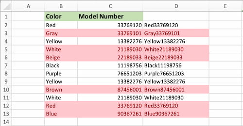
The final result will look like that! 

4. Highlight Consecutive Duplicate Values Only

Maybe you have a worksheet that has a few duplicates sprinkled in, but you only want to highlight the ones that are right next to each other in your dataset. There’s an easy way to do that, too!

• As usual, first select your data. That will be B2:B13 in this case.
• Select Conditional Formatting and Highlight Cells Rules.
• From the drop-down menu, choose Use a formula to determine which cells to format. 
• Enter the formula =OR(B2=B1,B2=B3)
• Select the formatting style you want and select OK.

Now, if your duplicate values aren’t consecutive, you won’t see any highlights. Head over to Sort & Filter, sort them alphabetically, and then you’ll see all the highlights pop up. 

If you try adding a non-consecutive duplicate – like a new row with Red up top – you’ll see that that one isn’t highlighted as it’s not beside the others.

There are more ways to highlight Duplicates in Excel, but these methods are simple enough for everyday use and usually take less than a minute once you’ve got a little practice. 

Do you have any other interesting ways to highlight duplicates in Excel? Let us know in the comments!