How to Create a Microsoft Excel Drop-Down List

Keeping your records organized is essential whether you’re running a business or taking care of the household. These days, there are a ton of apps you can use to keep track of daily to-dos, but they just can’t quite compare to the customization abilities and advanced features of Excel. One of those features is the Microsoft Excel drop-down list, which cuts down on the time it takes to input and track your data entries.

Drop-down lists can help Excel users narrow down options from a predetermined list and make finding information a little more intuitive. And luckily, making them is pretty simple – here’s how to do it and a few useful ways to implement them in your spreadsheets!

How to Create an Easy Microsoft Excel Drop-Down List: Step by Step

Let’s say you work in an office, and your manager wants to buy everyone lunch. She asks you to create a spreadsheet with all of your coworkers’ preferences. They can select either a sandwich, a salad, or pasta.

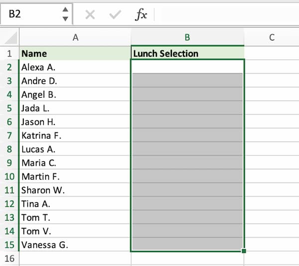
In the spreadsheet, column A lists the name of the employees, and column B lists their preferred lunch option.

You can download this example spreadsheet to practice: Data Validation List.

Step 1 – Select the range of cells where you’d like to enter the drop-down list. In this example, that would be B2 through B15.

Step 2 –  Navigate to the Data Ribbon options, and then select Data Validation.

Step 3 – You’ll see the Data Validation pop-up. Under the Allow drop-down list, select List.

Step 4 – In the Source section of the pop-up, enter your items separated by commas: Sandwich, Salad, Pasta.

Step 5 – Apply and close the dialog, and your drop-down list for the Lunch Selection column is ready!

You could share this spreadsheet with your coworkers and let them select whichever lunch they’d like.

Do You Need Formulas to Create a Microsoft Excel Drop-Down List?

As you can probably guess from above, the answer is no, you don’t need formulas to create drop-down lists. But, using them enables you to store your list of choices in cells (rather than manually entering them in the Source field as in the above example).

Storing the list of choices in cells makes it easier to adjust the list of choices in the future. For example, we simply change the values in the cells. This is faster than locating the input cells, selecting them, opening the Data Validation dialog, and editing the Source field list.

In the example above, we provided the list of choices by entering a comma-separated list in the Source field. However, we can also store our list of choices in a range of cells, and then use a simple formula to reference the range.

Storing List of Choices in Cells

We begin by entering the list of choices into cells. These can be on any worksheet in the workbook. For example, in the range A1:A3 on a different sheet named Sheet1:

Then, we select our input cells as before, and open the Data Validation dialog. We once again select List. But this time in the Source field, we use a formula to refer to the range A1:A3 on Sheet1, like this:

Note: Excel will enter the formula for you when you simply select the range of cells. However, you could type the formula manually if preferred.

We apply it, and bam:

If we think we may want to add more options to our list in the future, we can use a formula that refers to the entire column. So, instead of using this in our Source field:

=Sheet1!A1:A3

We would use this:

=Sheet1!A:A

That way, if we add new choices in column A, they will automatically be displayed in our drop-down.

A Couple of Things to Note When Creating Drop-Down Lists

Did you add a drop-down list to the wrong cell? No worries! You can easily copy + paste a cell with data validation into another cell of your choosing.

It can be a little hard to tell which cells have drop-down lists, so it’s a good idea to differentiate them with formatting like borders, cell colors, or a cell style.

If you want to copy a data validation cell, and paste ONLY the data validation settings (and not the formatting or cell value):

• Copy the data validation cell you want to paste.
• Select the cell (or cells) you want to paste the list into.
• On the Home Ribbon item, select Paste and then Paste Special.
• The Paste Special box will pop up. After selecting it, choose Validation from the Paste options menu.

You may also find yourself with several unformatted drop-down cells that you can’t locate. Don’t sweat it! There’s an easy way to find them:

• On the Home ribbon item, go to Find & Select and choose Go To Special. When the selections pop up, choose Data Validation.

• Note that you can select either All cells with Data Validation or only the Same cells with Data validation – meaning it’ll only highlight the cells like the one that’s currently selected. After you’ve made your selection, click OK, and all cells with that rule will be selected.

• After that, you can format them or apply a cell style so they don’t get lost again.

You can also set up a Defined Name to refer to your list of choices. You can do this by selecting the cells that contain the list of choices, typing the name into the Name Box (for example, MyRange), and pressing Enter on your keyboard. Then, in the Data Validation dialog’s Source field, you can write a formula that references the name, such as =MyRange.

Accidentally Deleting a Microsoft Excel Drop-Down List is a Little Too Easy…

So that’s why formatting can be so important!

If you do a normal paste into a cell with Data Validation, the drop-down list will be replaced by the Data Validation settings of the copied cell (if any). If the cell you copy has no Data Validation settings, then the pasted cell will now have no Data Validation settings. This is because when you Copy a cell, you are coping many attributes of that cell, including the Data Validation settings, cell value, and formatting. If the cell you copy has no Data Validation settings, then the destination cell will be updated accordingly and also have none.

If this happens, you can revert it if you quickly hit the undo button.

However, some best practices that can help you avoid this are to be sure to apply cell formatting or a cell style to your input cells to help you realize these cells have Data Validation applied. Also, when doing a Copy, get in the habit of doing a Paste Special Values (or Formula) so that you don’t Paste the Data Validation settings and formatting as well.

Microsoft Excel drop-down lists not only make navigating spreadsheets more intuitive, but they can also make them look sleeker and easier to understand.

Do you have any useful tips for making drop-down lists even better? Let us know in the comments!

Sample File