Create Dependent Drop-Downs with Spill Ranges

A while ago, I wrote about creating dependent (aka cascading, dynamic, or conditional) drop-downs using data validation. This is where you have a primary drop-down, and the choices in the related secondary drop-down depend on the selection made in the first drop-down. Well, this process became MUCH easier with the introduction of dynamic array functions and spill ranges. This is the first post in a series that explores dynamic array functions and spill ranges … strap in because it is going to be a fun ride 🙂

Objective

Our objective is to create two (or more) drop-downs, where the choices available depend on the selection made in the previous drop down(s).

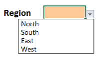
For example, we want to allow the user to select a Region from a drop-down, as shown below.

Then, based on the selected Region, the Rep drop-down should show only the corresponding Reps:

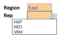
If a different Region is selected, the choices in the drop-down should reflect the reps in that region:

We can set this up using dynamic array functions and spill ranges.

Note: depending on your version of Excel, you may not have the dynamic array functions as shown below. At the time of this writing, it is available via O365 subscription only, and only if your update channel is set to Insiders Fast. These updates will be released to O365 users over time. These capabilities won’t be pushed out to perpetual license users of previous Excel versions (such as Excel 2019, 2016, and so on). If you’d like to get on the Insiders Fast update channel, check out your Update options in Excel. If you don’t have access to these features but would still like to create dynamic drop-downs, check out this post which uses features that have been available for the past 10 years.

Video

Narrative

We’ll explore dynamic array functions and spill ranges, and how to configure them to create depending drop-downs, using the steps below:

• Create Selection Choice Table
• Create Dynamic Choice Lists
• Create Drop-Downs

Let’s do this thing!

Create Selection Choice Table

The first step is relatively easy … you just create a table that stores all of the choices. The first column will contain the choices for the first drop-down, the second column for the second drop-down, and so on. Something like this:

Be sure this is saved in a Table (Insert > Table), and make a note of the table name in the Table Tools tab, or better yet, give the Table a descriptive name by using the Table Tools > Table Name field. I named my table Choices.

Note: You could create additional columns for additional drop-downs if needed.

Create Dynamic Choice Lists

This is where the process gets fun and uses dynamic arrays and spill ranges. These terms are relatively new to Excel users as I’m writing this post, so, let’s start with a brief background.

Dynamic Array Functions

Generally, we are used to writing Excel formulas that return a single value. Perhaps a sum, average, min, max, or count of some range of numbers. But, Microsoft recently revamped the Excel calc engine and introduced several new functions that return one or more values. Wait … what?

Yes … these newly introduced “dynamic array functions” return a dynamic array. A dynamic array … what? To simplify, think of an array as a way to store multiple values. Dynamic just means that the number of values returned can change as the arguments change.

For example, the SUM function returns a single value … we’ve been using that for decades. But, now we have a handful of new functions that can return multiple values, perhaps a list like 1, 2, 3, 4, and 5. But … Jeff … time-out. If a function returns multiple values, how can they be displayed in a single cell? Ah … insightful question, which leads to our next topic, spill ranges.

Spill Ranges

If a formula returns multiple values, they “spill” out into the cells below the formula. And, that spill range is dynamic. So, next time Excel calculates the formula, if more values are returned the spill range increases to include the values.

If you’d like to learn more about dynamic array functions and spill ranges, check out Bill Jelen’s book Excel Dynamic Arrays Straight to the Point which is a free download for a short time. He covers functions like SORT, SORTBY, FILTER, UNIQUE, SEQUENCE, and much more. More info here:

• https://www.mrexcel.com/products/excel-dynamic-arrays-straight-to-the-point/

Also, here is a great video for true Excel geeks that want to better understand the calc engine and arrays:

• https://www.microsoft.com/en-us/businessapplicationssummit/video/BAS2018-2140

Application

Now that we have a little background about dynamic array functions and spill ranges, let’s apply them to the task at hand.

Our goal in this step is to create one spill range for each drop-down. That is, to create two lists that will contain the choices to be displayed in the two drop-downs.

To create the list of choices for the primary Region drop-down, we need a unique list of the values in the choice table’s Region column.

This can be accomplished with the UNIQUE function, as follows:

=UNIQUE(Choices[Region])

The UNIQUE function returns a dynamic array of the unique values in the table’s Region column. Since the formula returns more than one value, the results spill into the cells below the formula as shown below.

We’ll use another dynamic array function to create the list of Reps, but first, let’s create the Region drop-down.

Create Drop-Downs

We’ll use data validation to create the drop-downs. Let’s start with the Region drop-down.

Region Drop-Down

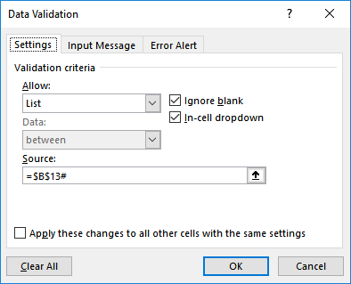
We select the desired drop-down cell, and use the Data > Data Validation command. This opens the Data Validation dialog, where we opt to Allow a List, and then in the Source field, we select the cell that contains our dynamic array formula. At this point, the Source field will contain a reference to a single cell, like this:

=$B$13

But, that is not what we really want. We don’t want our data validation drop-down to contain a single cell value … we want it to include all of the values in the spill range. So, to do that we add a # at the end of the reference. The hash/pound sign is used to create a spill reference, like this:

=$B$13#

This is shown in the dialog below.

After clicking OK, we see that our Region drop-down displays a list of Region choices … excellent!

So far so good … now we need to address the Rep drop-down.

Rep Choice List

We need to create the list of choices for the secondary Rep drop-down.

To do this, we’ll use another dynamic array function. If we think about this for a moment, we’ll realize what we need is a list of reps for the selected region. If we were looking at the Choices table, how would we accomplish this? For example, look at the table below and think of a way to get a list of Reps for the East Region:

We could apply a filter … that is, use the Region filter control and select East. The results are shown below.

Well, that is EXACTLY what the next dynamic array function does, and it is appropriately named FILTER.

The FILTER function applies a filter to a range and returns the filtered results.

In our case, we want the values in the Rep column where the Region is equal to East (or, the currently selected region). Assuming our Region selection (eg, East) is stored in C6, the formula is:

=FILTER(Choices[Rep],Choices[Region]=C6,"None")

You’ll notice the final argument “None” allows us to provide a value in the event the function returns no values.

We hit Enter and Excel displays the reps in the selected region. As the region changes, so does the rep list. Now, we just need to get that spill range into a data validation drop-down.

Rep Drop-Down

With the rep spill range created, we just add the secondary drop-down. We select the desired cell, and Data > Data Validation. We once again allow a List and the Source is the dynamic array formula cell followed by #, as shown below.

With that complete, we now have a primary Region drop-down, and the secondary Rep drop-down choices depend on the region selected. Yay!

If you have any other related tips on depending drop-downs or dynamic array functions, please share by posting a comment below … thanks!

If you need to have more than two drop-downs, it is no problem … the sample file has a sheet with three drop-downs.

Download sample file: DependentDropDowns.xlsx