Unpivot Excel Data

Excel easily summarizes flat, tabular data. When data is stored in a crosstab style format instead, Excel users have to spend a bit of time preparing the data for use. There are many ways to accomplish just about any Excel task, but in this post, I’ll demonstrate how to quickly unpivot the data. Thanks to Patrick who submitted this question.

Objective

Before we dig into the mechanics, let’s be sure we are clear about the data formats and our objective.

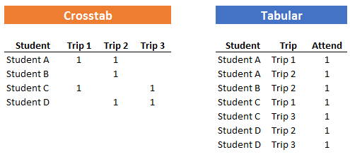
Here is an example of flat, tabular data:

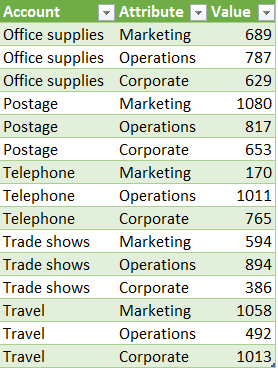
Here is an example of the same data stored in a crosstab style format:

We can easily convert tabular data into a crosstab format using a PivotTable. But here, we want to do the opposite. We want to unpivot the data, converting it from a crosstab format into a tabular format.

Note: please note that unpivoting the data is not the same as transposing it. Transposing the data would place departments in rows and accounts in columns. If you need to transpose instead of unpivot, check out this Excel University blog post instead.

Here is another example that shows students and the trips they have attended.

And one more example that tracks who is assigned to various tasks.

Now that we have our bearings and can visually see our objective, let’s work through the details.

Unpivot

The unpivot command is available without any additional downloads in Excel 2016 for Windows. If you are using a different version, you may need to first download the free Power Query add-in from the Microsoft site. At the time I’m writing this, it is available from the link below.

The four easy steps we’ll use to unpivot our crosstab data are:

• Store the crosstab data in a table
• Get & Transform From Table
• Unpivot
• Load

We’ll take them one at a time.

Store the crosstab data in a table

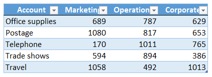
First, we need to ensure that our crosstab data is stored in a table. If it already is, you can skip this step. Our data isn’t stored in a table, and it currently looks like this.

To convert it into a table, we select any cell in the data range and click the Insert > Table command. Now, it is stored in a table and looks like this.

Hey, that was pretty easy. Let’s move to the next step.

Get & Transform From Table

The next step is to use the Get & Transform From Table command. Again, this is built-in beginning with Excel 2016 for Windows. If you have a different version, you’ll want to download and install Power Query using the link below, and note that the navigation may be slightly different from the screenshots presented below.

First, we select any cell in the table. Then, we click the following Ribbon command located in the Get & Transform group.

• Data > From Table

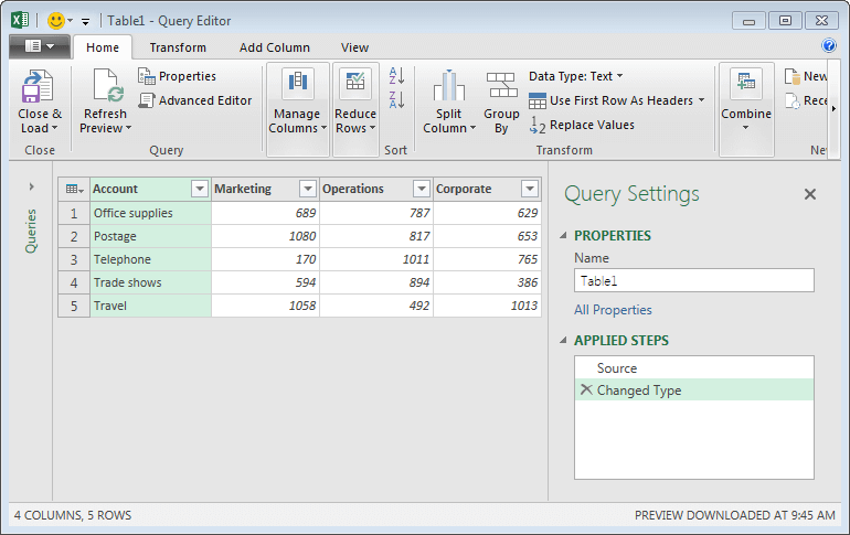
This opens the Query Editor, as shown below.

Hey, that was pretty easy…let’s take the next step.

Unpivot

Before we use the unpivot command, we first need to tell Excel which columns we’d like to unpivot. To do this, we can select the first column we want to unpivot, hold down the Shift key, and then click the last column. The results are shown below.

Note: if you would like to undo a step in the Query Editor, you click the x in the Applied Steps list box.

Now that we have identified which columns to unpivot, we can use the unpivot command. The unpivot command is located on the Transform tab. Since the Ribbon dynamically sizes itself based on the dialog size, you may see the unpivot columns command with a text label, like this:

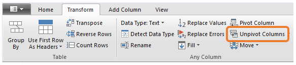
Or, it may appear without a text label, like this:

Just click the command icon, and bam, Excel unpivots the data, as shown below.

Hey, that was pretty easy! The final step is to load the data back into our workbook.

Load

With the data unpivoted, we just need to get it back to our workbook. To do so, we use the Close & Load command on the Home tab. Excel drops the unpivoted data back into our workbook, as shown below.

That was easy!

The unpivot command is but one of the many powerful capabilities in the Query Editor dialog. If you retrieve data from external sources and perform data transformations often, you’ll definitely want to investigate the additional commands.

Additional Resources

• Sample file: Unpivot
• Power Query download: https://www.microsoft.com/en-us/download/details.aspx?id=39379