Excel Rules

Two enhancements introduced in Excel 2007 may have slipped past you: multiple condition sum with SUMIFS and Tables (not Pivot Tables). It’s my hunch that once you discover them, you’ll fall in love with them the way I have.

Please note: this Author’s version contains additional screenshots and info. For the Published version, please visit calcpa.org.

Multiple Condition Sum
The SUM() function, which adds all cells in a range, is probably your most favorite and most used function. Sometimes, however, we only want to include rows that satisfy a condition. For example, only those rows where account equals “cash.”

Historically, performing a conditional sum that has only one condition was easily accomplished with the SUMIF() function. But that function does not allow multiple conditions, such as including those rows where account equals “cash” and where period is equal to “January.”

In versions of Excel prior to 2007, creating a multiple condition sum requires the use of complicated functions, like SUMPRODUCT() or Array formulas. However, Microsoft introduced the SUMIFS() function in Excel 2007, which supports multiple conditions. I’ll demonstrate one very cool use of this function.

Let’s assume you have a client that uses QuickBooks and you need a report that QuickBooks doesn’t provide exactly right. Let’s also assume you would like an efficient way to export transaction data from QuickBooks and have Excel formulas automatically pull the right values to the right cells. This is now easy, thanks to the SUMIFS() function.

For this example, we have a workbook called report.xlsx

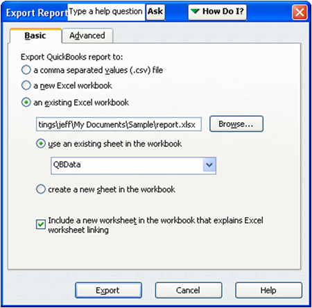
The workbook contains a worksheet named QBData, which represents the “landing page” that accepts direct QuickBooks exports. QuickBooks supports the export of virtually any report or transaction list into an Excel format, but the best trick is to export a QuickBooks report to an existing workbook and to a specific worksheet within the workbook, as seen in the screenshot below.

This technique makes recurring processes more efficient. Once you export the QuickBooks data into the QBData worksheet each period, the smart formulas on the report worksheet will automatically pull the correct values from the QBData sheet. That brings us to a smart formula, the SUMIFS() function. The syntax of the SUMIFS() function follows:

=SUMIFS(sum_range,criteria_range1,criteria1,…)

Where:

• sum_range is the range of cells that you want to add.
• criteria_range1 is the range of cells that has the values to compare to criteria.
• criteria1 is the cell that contains the criterion.

Note: You may specify up to 127 criteria_range/criteria pairs.

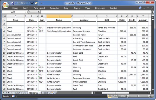
Let’s say you have a memorized report in QuickBooks that you want to export and summarize each period. Further, let’s assume that a PivotTable isn’t a good fit for this project because you are creating a client deliverable and not simply analyzing data. An example of the Quickbooks transaction export is shown below.

Perhaps our report needs to show the total Debits (col P) for those rows where Type (col D) equals “Check.” Or, our report needs to show the total Amount (col T) by Type (col D). These are easily produced via the SUMIFS() function.

To get us warmed up, let’s add the values in the Debit column and include only those rows where Type equals “Check” and where Name equals “Bayshore Water.” Conceptually, you would want to sum the values in the Debit column (P) where Type (col D) equals the value “Check” and where the Name column (J) equals “Bayshore Water.” That logic translates into the following SUMIFS() function:

=SUMIFS(P:P,D:D,“Check”,J:J,“Bayshore Water”)

Where:

• P:P is the column reference that has the values to add (the Debit column).
• D:D is the column reference that has the first criteria (the Type column).
• “Check” is the value that D:D must equal to be included in the sum total.
• J:J is the column reference that has the second criteria (the Name column).
• “Bayshore Water” is the value that J:J must equal to be included in the sum total.

Making the formula more useful, we would swap the hard-coded function arguments “Check” and “Bayshore Water” with cell references as shown in the screenshot below.

We can then fill the formula down to create a simple summary report. Next period we can simply export the QuickBooks transaction list into the QBData sheet and the report is automatically updated with the new data.

The next example demonstrates creating monthly columns. For this trick, you’ll need to be familiar with a function called EOMONTH(), which returns the last day of the month. This function has two arguments: any date and the number of months from date.

For example, to return the last day of the date in cell A1, the function is =EOMONTH(A1,0). To return the last day of the next month: =EOMONTH(A1,1). To return the last day of the previous month =EOMONTH(A1,-1). You get the idea. To create a report that has monthly columns, you include the date column (col F) in the SUMIFS() function.

Say you wanted to sum the Debit column (col P) for all rows where Type (col D) equals “Credit Card Charge” and where the Date (col F) is in the month defined in cell A1. You would create the following function:

=SUMIFS(P:P,D:D,”Credit Card Charge”,F:F,”>=”&A1,F:F,”<=”&EOMONTH(A1,0))

Where:

• P:P is the column that has the numbers you want to add, the Debit column.
• D:D is the first criteria range, Type.
• “Credit Card Charge” is the first criteria, to be compared to column D:D.
• F:F is the second criteria range, Date.
• “>=”&A1 is a concatenation of the comparison operator “>=” (greater than or equal to) and the date in A1.
• F:F is the third criteria range, Date.
• “<=”&EOMONTH(A1,0) is a concatenation of the comparison operator “<=” (less than or equal to) and the last day of month for the date in A1.

To see it in action, check out the screenshot below. Note the use of absolute cell references ($) so that as the formula is filled down and right it continues to work as expected.

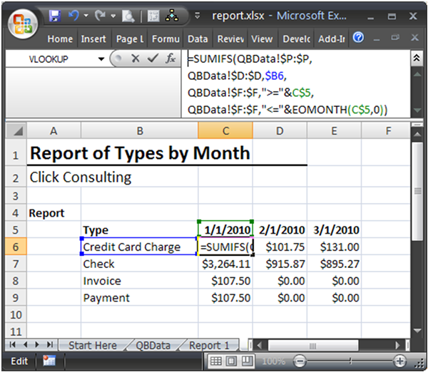
Next period, simply export the QuickBooks transaction list into the QBData sheet and the smart SUMIFS() functions pull the values into the right spot—automagically!

Tables
Think of a Table (not to be confused with Pivot Tables) as a continuous range of cells that has many rows and many columns that are filled with values or formulas. Starting with Excel 2007, you can convert a standard range of data into a Table, and Tables have special properties. There are many superpowers that Tables have, but the best three are:

• Automatically adjusting range.
• Structured references.
• Auto-fill-down for formulas.

Automatically adjusting range
A Table automatically extends when you type data in cells directly adjacent to the Table. So, if you type values in cells directly under the Table, the Table automatically extends to include the new data that you type. Let me walk through how we can apply this to our advantage.

Typically, in formulas, ranges are referred to with range references like A1:B10. If you enter new data in the row under the range reference you have to manually update those formulas to include the newly inserted data. Since Tables automatically expand themselves to include the new data, as long as you write your formulas using the Table name (rather than the row/column reference) your formulas will automatically include the newly inserted data. That saves you time since you won’t need to update the formulas—and it makes your formulas bulletproof.

To demonstrate, consider the “normal” data range shown in the screenshot below.

Once you select a cell in the range, and then Insert > Table, your traditional data range is converted into a Table, as seen in the screenshot below.

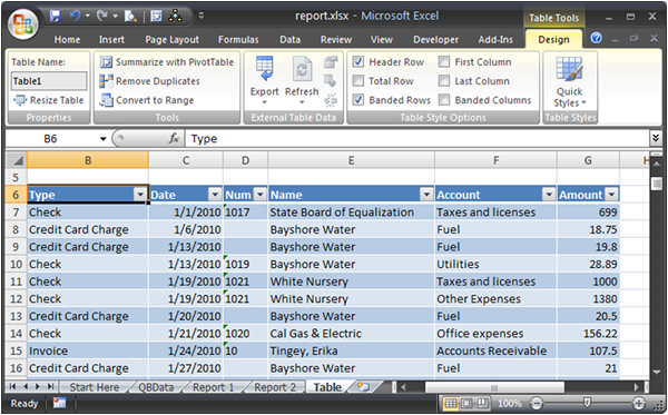
You’ll notice some fancy formatting and the addition of a new tab in your ribbon called “Table Tools.” One setting is called “Table Name,” which defaults to Table1, but is easily modified.

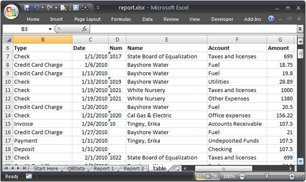
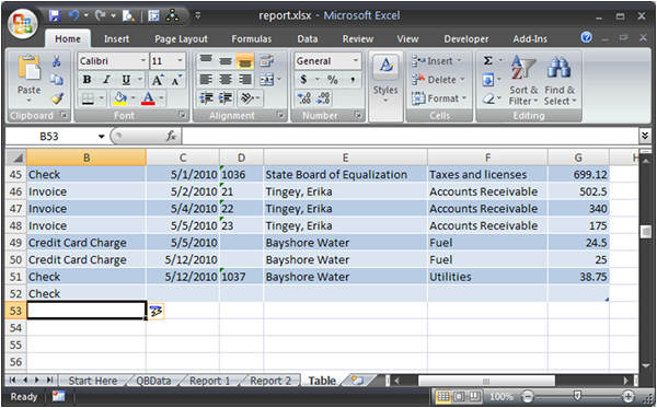
Now, to refer to this data Table in formulas, instead of referring to it with row/column references like B6:G51, simply use the Table name in your formulas, “Table1” in this case. As data is entered directly below the Table (in row 52), the Table automatically expands to include the new data and also extends the name Table1 as seen in the screenshot below.

Thus, any formulas that use Table1 will continue to work on the range, including the newly inserted data. This is a huge feature of Excel 2007. But, this feature just keeps getting better. Let’s explore structured references.

Structured references
Referring to data inside of a Table is easy. Do you remember the SUMIFS() function we played with above? We used standard cell references in the examples. However, if we use SUMIFS() on a Table, we can use structured references.

For example, we can refer to a column of a Table by using the syntax TableName[ColumnName], in this case Table1[Amount] to refer to the Amount column inside Table1. Applying this to SUMIFS() formulas becomes quite easy. For example, if we wanted to sum the Amount column and only include those rows where Type equals Check and where Account equals Utilities, we would use this elegant syntax:

=SUMIFS(Table1[Amount],Table1[Type],“Check”,Table1[Account], “Utilities”)

Formulas that use a Table’s structured references are more reliable and more flexible, since they automatically adjust if values shift into other columns. There are additional structured references available, including:

• TableName[ColumnName] to refer to a column.
• TableName[#Totals] to refer to the total row.
• TableName[#Headers] to refer to the header row.
• TableName[#ThisRow] to refer to the current row.

With Excel 2007’s new auto-complete feature, as you type in the table name and then an open square bracket, Excel will show you the structured reference options as shown in the screenshot below.

Auto-fill-down formulas
When you enter a formula into a column adjacent to a Table, Excel fills the formula down and will automatically fill it down as new data is added under the Table. This saves time and makes the Table more reliable.

Used properly, Excel streamlines recurring processes and generally helps to automate mechanical tasks. I hope you enjoy these two new gifts from Microsoft, and as you know…Excel rules!