WORKDAY Function

When you need to compute a future date and exclude weekends, you may want to consider exploring the WORKDAY function. In this post, we’ll use the WORKDAY function to prepare a simple project plan and then display it with a Gantt chart.

Objective

We have a project that we are managing and it has several tasks. We know the start day and the number of workdays each task takes to complete. We want Excel to compute the end date for each task. We can’t simply add the start date and the number of days because that would include weekends. We need to exclude weekends from the equation.

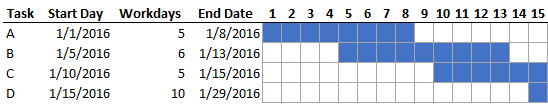
Once Excel computes the end date, we’d like a simple way to display the project timeline visually, in a Gantt chart. The end result should look like this.

These are the steps we’ll use to complete our workbook:

• Compute the End Date with the WORKDAY function
• Set up the Gantt chart
• Conditional formatting formula
• Cosmetics

Let’s get to it.

WORKDAY

First up, computing the End Date with the WORKDAY function. Task A starts on 1/1/2016 and it is scheduled to take 5 workdays. If we were to simply add these values together, we would get 1/6/2016, an incorrect End Date. This is because we want to exclude weekends from our calculation. This is where the WORKDAY function can help. It computes the End Date based on a start date and the number of workdays, and excludes weekends. It can additionally exclude a list of holidays if needed.

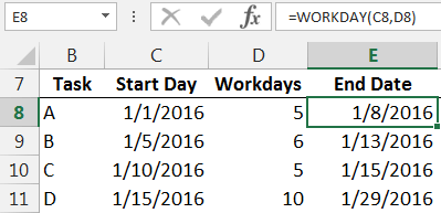
Since our Start Date is stored in C8, and the number of workdays in D8, we can write the following formula into E8:

=WORKDAY(C8,D8)

The WORKDAY function returns a date of 1/8/2016…perfect. We fill the formula down for all tasks as shown below.

Now let’s move to the Gantt chart.

Gantt Chart

The Gantt chart is created with conditional formatting. Before we jump to the mechanics, let’s consider what we are trying to accomplish conceptually.

We would like to fill the cells blue when the day is between the start and end date (inclusive). For example, if we look at column F, the day is 1/1/16. We want to fill the cell blue for Task A since 1/1/16 is between the Start Day (1/1/16) and the End Date (1/8/16). We don’t want to fill the remaining cells in column F for the other tasks since 1/1/16 does not fall between their start and end dates. So far so good? This same logic carries right through all of the columns. When the day falls between the start and end dates, we want to shade the cell blue.

The good news is that we can apply this logic to Excel with the conditional formatting feature.

Conditional Formatting

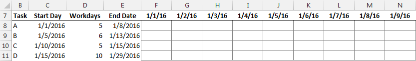
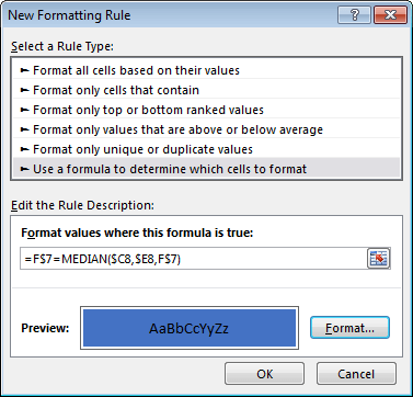
To begin, we select all of the cells in the Gantt chart range, that is, F8:AJ11. Then we select Conditional Formatting > New Rule. In the New Formatting Rule dialog, we opt to “Use a formula to determine which cells to format” and, assuming that cell F8 is the active cell within the selected range, we enter the following formula.

=F$7=MEDIAN($C8,$E8,F$7)

A couple of notes about this formula. First up, the MEDIAN function is designed to return the middle value of its arguments. We use the start date, end date, and day values as arguments, and it will return the middle date. We compare that middle date to the day in F7, and if it is equal, then the formula will return TRUE and apply the selected formatting. If F7 is not the middle date, then the formula returns FALSE and Excel does not apply the conditional formatting.

Next, we need to pay attention to the cell references used. We need to imagine that the formula will be filled through the entire selected range. That means we need to pay attention to absolute and relative references. Starting with the date stored in F7, as the formatting formula is filled down, we need the reference to stay locked onto the same row, and as it is filled right we want the column reference to update accordingly. So, we used the mixed cell reference style F$7, which is absolute row (7) and relative column (F). For the start and end dates stored in C8 and E8, as the formatting formula is filled down we want the row reference to update, but as it is filled right we want the column reference to stay put. So, we use the mixed cell reference style $C8 and $E8 which provides a relative row and absolute column.

Note: As an alternative to using the MEDIAN function, we could have used the following formatting formula instead:  =AND(F$7>=$C8,F$7<=$E8)

With our conditional formatting formula complete, we simply use the Format button to select the type of format to apply. I just used a simple blue cell fill. The resulting dialog is shown below for reference.

With conditional formatting applied, our Gantt chart is looking good!

Now for a few cosmetic updates.

Cosmetics

Instead of showing the full date, we just want to show the day number. So, we select the Gantt chart date header values, and apply the following custom cell format.

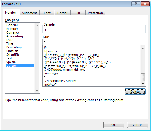
The d in the Type field tells Excel to display the day number only. We then change the column width for the Gantt chart columns to 2, optionally format the cell borders gray, and the updated project tracker is shown below.

Alright, I think we achieved our objective!

If you have any other uses for the WORKDAY function, or other approaches to Gantt charts, please share by posting a comment below…thanks!

Resources

• Workday
• Excel University Conditional Formatting post