VLOOKUP on Two or More Criteria Columns
If you have ever tried to use a VLOOKUP function with two or more criteria columns, you’ve quickly discovered that it just wasn’t built for that purpose. Fortunately, there is another function that may work as an alternative to VLOOKUP depending on what you want to return.
Video
Multi-Column Lookup Objective
First, let’s confirm our objective by looking at a sample workbook. We have exported some information from our accounting system, and it is basically summarizes the transaction totals for the month by class and by account. A sample of the export is shown below:
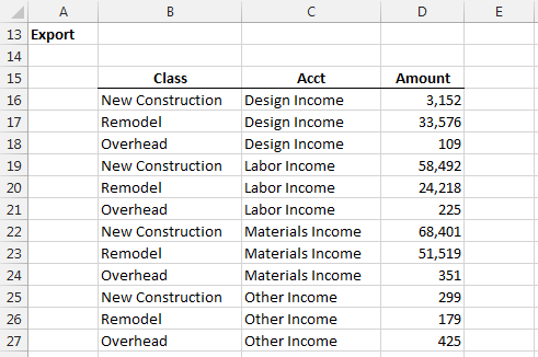
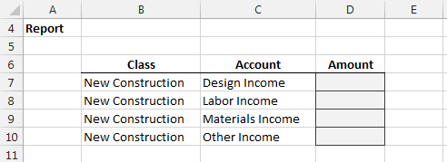
From this exported data, we would like to retrieve selected amounts based on the class and account columns. We want to retrieve the amounts and place them into our little report, pictured below:
If you are familiar with the VLOOKUP function, it feels natural to try to build the report with this function because, after all, this is a lookup task. And, lookup tasks are best solved with traditional lookup functions…right? Well, it depends. It depends on what you are trying to retrieve.
Conditional Summing for Lookups
If you are trying to retrieve a numeric value, such as an amount, then a traditional lookup function may not be your best bet. Here’s why. Beginning with Excel 2007, Microsoft included the conditional summing function SUMIFS. This multiple condition summing function is designed to add up a column of numbers, and only include rows that meet one or more conditions. Are the dots starting to connect yet?
If we apply this idea to our task at hand, we would quickly realize that we could use this conditional summing function to retrieve our report values.
The first argument of the SUMIFS function is the sum range, that is, the column of numbers to add. In our case, the column that has the value we wish to return. The remaining arguments come in pairs: the criteria range and the criteria value.
It is helpful to think about the function in these terms: add up this column (argument 1), only include those rows where this column (argument 2) is equal to this value (argument 3), and where this column (argument 4) is equal to this value (argument 5), and where…and so on, up to 127 pairs.
Thus, to populate our report, we’ll retrieve the amount values from the export, and match the class and account columns, as shown below.
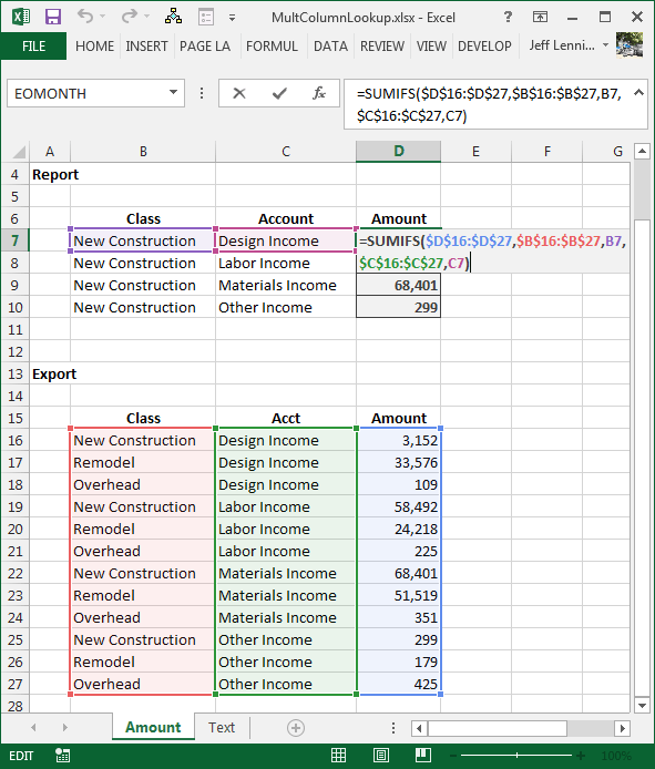
If there happen to be multiple rows with the same class and accounts, then the SUMIFS function would return the sum of all matching items.
As you can see, if the value you are trying to return is a number, then the SUMIFS function makes it simple to perform multi-column lookups. But, what if the value you are trying to return is not a number? Well, then you’ll need to use a traditional lookup function as discussed below.
Using VLOOKUP with SUMIFS Method
One method is to use VLOOKUP and SUMIFS in a single formula. Essentially, you use SUMIFS as the first argument of VLOOKUP. This method is explored fully in this Excel University post:
https://www.excel-university.com/multi-column-lookup-with-vlookup-and-sumifs/
Using VLOOKUP with CONCATENATE Method
If you are trying to return a text string rather than a number, or are using a version of Excel that doesn’t have SUMIFS, then you are probably stuck with using a traditional lookup function such as VLOOKUP along with the CONCATENATE function to generate a single unique lookup column. This approach is fairly well documented, but the basic idea goes like this: create a single lookup column first, and then use VLOOKUP.
Our example will be an employee list, as illustrated below:
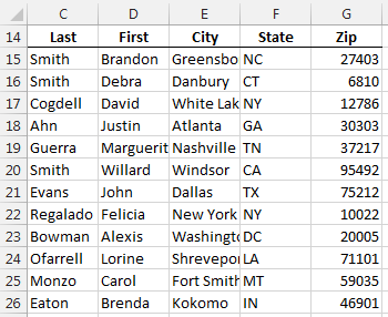
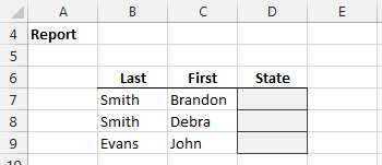
We need to retrieve the state from the employee list for our little report shown below:
Since the value we are trying to return, the state, is a text string and not a number, we are precluded from using the SUMIFS function. Thus, we’ll need to go old-school with VLOOKUP and CONCATENATE.
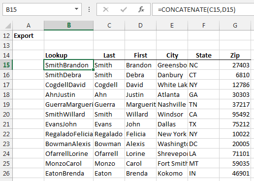
We start by building a helper column that basically creates the combined lookup values. This can easily be accomplished with the CONCATENATE function or the concatenation operator (&). This new lookup column is illustrated in column B below:
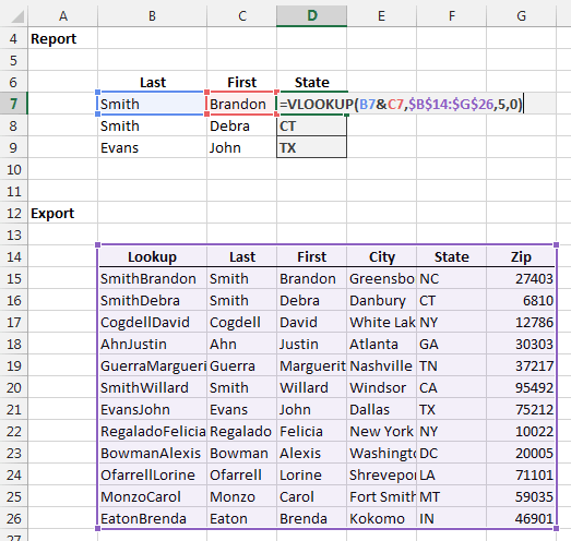
Now we have a single lookup column that can be used with a traditional lookup function such as VLOOKUP. The report can be populated by looking up the combined names within the new lookup range, as shown below:
This same approach can be used when two, three, or more lookup columns need to be considered.
FREE: Excel Speed Challenge
If you enjoyed this post, please check out our free Excel speed challenge.

Watch one short Excel video a day for 5 days. Total video time is only 45 minutes. Learn the Excel skills that can help you save an hour a week.
Conclusion
In addition to being able to perform multi-column lookups when the return value is numeric, the SUMIFS function has additional benefits when compared to traditional lookup functions. For example, it returns zero when no matching value is found, it returns the sum of all matches, it supports comparison operators, and it won’t break when a new column is inserted between the lookup and return columns.
So, when you are about to bust out the VLOOKUP function to do a lookup task, consider using SUMIFS instead. Believe it or not, the SUMIFS function makes a wonderful lookup function.
If you have any other preferred approaches to multi-column lookups, we’d love to hear more…please post a comment below.
Sample File
If you want to play with the workbook used to generate the screenshots above, please feel free to download the sample file:
Excel is not what it used to be.
You need the Excel Proficiency Roadmap now. Includes 6 steps for a successful journey, 3 things to avoid, and weekly Excel tips.
Want to learn Excel?
Our training programs start at $29 and will help you learn Excel quickly.
Really helpful, Thanks!
Thanks a ton.. Very simple and easy to use solution for both numbers and text strings! It helped me solve a problem in minutes Great job guys…
My only issue with this is when one of the columns has more than one word. I can’t include any spaces.
Customers Table
A2 (Lookup): CompanyCanadaVancouver
B2 (Account): 1234
C2 (Company): CompanyCanada
D2 (Branch): Vancouver
Contacts Table
A2 (Account): =VLOOKUP([Company]&[Branch],Customers,2,TRUE)
B2 (Company): CompanyCanada
C2 (Branch): Vancouver
It would be nice if I could do this with a space between Company & Canada.
Amy,
Hmmm…I tried it here with a space between Company & Canada, and it seemed to work. Here are the values I used in my tests:
Customers Table
A2 (Lookup): Company CanadaVancouver
B2 (Account): 1234
C2 (Company): Company Canada
D2 (Branch): Vancouver
Contacts Table
A2 (Account): =VLOOKUP([Company]&[Branch],Customers,2,TRUE)
B2 (Company): Company Canada
C2 (Branch): Vancouver
The VLOOKUP function returned the 1234 value successfully. I’m thinking perhaps it may be a different issue? For example, a common issue is that the export may actually include trailing spaces. If so, you can use TRIM to remove excess spaces. Another idea is that you can concatenate a space into the VLOOKUP function if needed, such as VLOOKUP(A1&” “&A2…).
Also, I’d want to confirm that the values in both tables include, or exclude, the space. For example, that C2 in the Customers Table has a space (Company Canada) as well as the corresponding value in the Contacts Table (B2, Company Canada).
I hope these ideas are helpful!
Thanks
Jeff
It’s not exactly applicable here but I’ve found that ‘sumifs’ can be done without SUMIFS, so to speak.
For Smith sales in NC – using an added fictional Sales column (H) and changing the States so that some are matching (Changing Willard Smith to NC)….
{=SUM(IF(C15:C26=B7,IF(F15:F26=D7,H15:H26,0),0))}
You need Shift&Enter or {} to activate the formula.
Marc,
Thanks for sharing your array formula alternative!!
Thanks
Jeff
How would i do it if i wanted to look up 3 columns?
Example A is the convenate of b&c.
B=Article
C=PO
D=Date
E=QTY
If the item you want to return is numeric, then I recommend using SUMIFS and just add another criteria_range/criteria_value pair of arguments. If the item you want to return is a text string, then I recommend using concatenate to combine the lookup columns.
The sample file has example formulas for reference.
Thanks
Jeff
Fantastic – thank-you
Table No Start date End date Society Name
1 1/7/2015 3/7/2015 ABCD
2 2/7/2015 5/7/2015 PQRS
1 5/7/2015 7/7/2015 ABCD
1 7/7/2015 10/7/2015 XYZ
HI ,
My query is that if i have to develop a vlookup with multiple criteria such that if Table No is 2 and the satart date and End date lies between the mentioned dates then the society name should be pulled out.
Can you please help!!
Amit,
Since the SUMIFS function is designed to return a number, and not a name such as the society name ABCD, we can’t use it directly…however…we can use it along with a helper column. Here is the basic idea. You create a new helper column in the data range, something like “RecordID” or “ID” which is a unique number for that row, such as 1, 2, 3, 4, and so on. Then, assuming that the conditions can only be met by a single row, you can use the SUMIFS function with multiple conditions to return the RecordID to a cell, say A1. Then, you can use a VLOOKUP that finds the RecordID stored in A1 in the lookup range to return the society name. You could even combine the SUMIFS and VLOOKUP in a single formula with something like this: =VLOOKUP(SUMIFS(sum_range, criteria_range1, criteria1, …), lookup_table, 5, 0)
Hope this idea helps!
Thanks
Jeff
Well, I couldn’t have dumped into a better website looking in search for the excel solution. Thanks a lot!!!
I need to show the rank ABCDE on Quality performance and rank abcde on productivity performance.is it possible?
Experience Quality Performance Rank
– 20% E
1 80% D
3 85% C
6 90% B
12 95% A
Productivity Performance Rank
49% D
50% C
75% B
95% A
Hey Jeneth
It sounds like you just need to sort the data:) Select any cell in your table and apply sort/filter arrows with Ctrl+Shift+L. Then you can select the option you want:)
Hope that helps,
Kurt LeBlanc
PERFECT PERFECT PERFECT
THANKS A TON
What if i have two columns of amount to sum? Any suggestion? the sum range doesn’t appear to work with multiple columns…
Saved me a lot of time. superb
Hello Mr. Lenning,
This simple solution to the problem that I thought it had become a puzzle, is incredibly helpful. Now, I was wondering, just for aesthetics, could it be posible for your example to just show an item e.g., Design Income, only once in the drop down list, the same with all items in the drop down lists. Just once.
It sounds like you are trying to create a drop-down with a unique list, even if the source may have multiples of each item. I walk through one solution in the following post.
https://www.excel-university.com/unique-data-validation-drop-down-from-duplicate-table-data/
I hope it helps!
Thanks
Jeff
Perfect Thanks Sir.
Hi Jeff,
Could you please help me?
I have a table and it’s got Hotel Name, Basis – Bed & Breakfast (BB) or Half Board (HB) and a Price list on two columns with 1st column with the Single Rate Prices and Then 2nd column with Double Rate Prices. I need to calculate using the drop down lists 1st the Hotel Name then the Basis and then by Single or Double. Can I use “IF” formula and “VLOOKUP” formula for this? As i’m getting a error on the formula i wrote. could you please help me to write the code. here is the formula i wrote…. ‘=VLOOKUP(A10,Table1,IF(Table1[[#Headers],[Single Room Rate]]=”Single”,Table1[Single Room Rate],Table1[Double Room Rate]),1)
Thanks,
Sampath.
It is very Helpful. But can you help me.
1) if 2 Vlookkup conditions’ Colum Ref. is…. Number & Number…………IT IS HELPFUL.
1) if 2 Vlookkup conditions’ Colum Ref. is…. TEXT & TEXT…………IT IS HELPFUL.
. But I can’t use the formula if Volookup …if …One Condition is TEXT,… and another Condition is DATE.
Please Help me.
Hey Sandeep,
I think you’ll have to nest the SUMIFS in a VLOOKUP like this:
https://www.excel-university.com/multi-column-lookup-with-vlookup-and-sumifs/
Dates can be recognized as numbers in Excel.
Let me know if that helps:)
Kurt LeBlanc
Why did they create a function to sum based on two or more criteria but no function to lookup based on two or more criteria?
Hey Bill
I can’t answer as to why Microsoft didn’t, but they may be developing it as we speak. They make improvements all the time.
I can’t wait to see what they do next!
Kurt LeBlanc
Can we loop vlookup in a single cell, like to search 2 thing/ item in a single vlookup command
Hey Salim
Unfortunately you can’t with VLOOKUP but SUMIFS can if the result is a number you need. Mr. Jeff has a great blog on this topic:
https://www.excel-university.com/multi-column-lookup-with-vlookup-and-sumifs/
Look into this. It’s pretty interesting how i works:)
Let me know how this works,
Kurt LeBlanc
Hello sir I have one question I will send you excel sheet kindly send me your email address
[email protected]
Hey Sanum
I can help you on here, but I don’t want to give out my email.
Thank you
Kurt LeBlanc
Thank you! This was very helpful
Thank you so much!
I was as at complete standstill trying to figure out how to do this… You way worked perfectly!
Pondered the problem for a week, your solution took 5 minutes…
Awesome, glad this post helped 🙂
Jeff,
A really helpful post… i just have one question on this, the original SUMIFS formula works perfectly, except for the fact that one of my criteria columns has positive AND negative numbers in… it recognises the positive numbers and returns the correct value at the end, however the negative criteria values with the same syntax arent recognised and just return a zero.
Is there any way around this?
Appreciate anything you may have
Hey, this was great!
I have one question though and I’m not sure if this is the right place to ask, but what if I was looking for specific text? So if I wanted to fill a cell with something like Family Room. Assuming the number 203 pertains to the family room, how would I get information from a “Label” column that contains HE-203, how would I write my formula so that the target cell displays “Family Room” when referencing the Label column that has HE-203 on the same row?
Hi Jeff,
I am trying to find a formula to resolve the following:
Column A has three criteria and column B has five criteria. I would like to have the summed value in column C for each criteria in column A that satisfies one or more of the criteria in column B, and return the value if it is >0.
Thanks.
Really insightful stuff Jeff. Thanks for sharing.
Hello,
I have a numeric data set which is similar to the example shown above.
I tried the SUMIFS function on my following data set.
Column A –> Eng Spd –> 750, 1000, 1400, 1800, 1400, 750, 1000
Column B –> Eng Trq –> 0, 40, 50, 70, 80, 20, 60
Column C –> Point –> 10, 42, 56, 87, 63, 94, 23
I wish to retrieve the corresponding Point values in Column G for the subset of Eng Spd and corresponding Eng Trq values as shown below.
Column E –> Eng Spd –> 750, 1400, 1800, 1000
Column F –> Eng Trq –> 20, 50, 70, 60
Column G –> Point –> ?, ?, ?, ?
I tried as shown above, however, I got the Point values as 0 in all the 4 cases of my subset.
Kindly help!!!
Hi there,
I am looking to create a crop search spreadsheet that matches potential crops to a set of criteria for any given farm.
For example a farm at Nyngan Australia has average rainfall 460mm, soil PH5.5, minimum temperature 0 degrees Celsius, soil type is loam, I want an ANNUAL crop, that is a LEGUME.
How can I code a list of potential crops into a vault sheet that when I type in my selection criteria for the farm it only displays the crops from the vault that match the criteria entered ie if RYEGRASS needs 650mm rainfall it will be not displayed but BUFFEL GRASS only needs 300mm rainfall therefore is a match.
I am looking for up to 10 columns to be searched not just text but Y/N criteria and words as well is this even possible?
Hi,
I have multiple sheets(180 Sheet) having the Revenue and Cost figures of the Outlet along with Their Outlet code, Month, Heads of Expenses and Revenue.
How can i drive formula for making of Outlet wise summary, with lookup condition of Outlet code, Months and Particulars.
If i change the Months , all data will change accordingly.
Can we also use INDIRECT Function
Can you explain this same problom of 2 way lookup with match index
Hi
i have Two different sheet i want check as per details given below
1st: Party Name (If Party Name Match )
2nd : than Bill Number
3rd : Bill amount
Above 3 parameter match then reply “Yes” other wise Reply “NO”
What formula i can use
Good Day to you, I have a question.
I need a Vlookup formulas for 2 sheets, base on two criteria on sheet2. First the date (A1), then the Item code (B1), to get the total amount at sheet1.
hope to get some help from u.
Thanks you so much
Hello,
This page was really helpful is solving a multi-criteria lookup problem for me without spending a lot of time looking. Really appreciate this page!
Dear all,
i need help in extracting data from multiple columns through vlookup formula
below is my table
Hotel name period DBL TPL Quad Meal
A 01-01-2021- 30-01-2021 100 200 300 BB
A 01-02-2021- 30-02-2021 100 200 300 BB
A 01-03-2021- 30-03-2021 100 200 300 BB
B 01-01-2021- 30-01-2021 100 200 300 BB
B 01-01-2021- 30-01-2021 100 200 300 BB
B 01-01-2021- 30-01-2021 100 200 300 BB
C 01-01-2021- 30-01-2021 100 200 300 BB
C 01-01-2021- 30-01-2021 100 200 300 BB
C 01-01-2021- 30-01-2021 100 200 300 BB
D 01-01-2021- 30-01-2021 100 200 300 BB
D 01-01-2021- 30-01-2021 100 200 300 RO
so when i want to extract details for hotel A it should give me all the details for all periods concerning to hotel A
i tried to extract with Vlook up formula but its fetching only one row (first row only)
That really helped me! well written and right to the point. thanks!
Can I use AND function to compare two vlookups?
Brilliant. I was searching all over to figure out how to do this, and I even use SUMIFS all the time. Never occurred to me to use it in this way.
Still really helpful (particularly the downloadable example) in 2025!