VLOOKUP Hack #9: Partial Match
Let’s say we want VLOOKUP to match the lookup value “North Region” with “North Region Subtotal” stored in the lookup range. We started this series by looking at the 4th argument. We know it can be TRUE or FALSE. FALSE means exact match and TRUE means approximate match. So, what exactly is an approximate match? Well, as you may have guessed, we’ll dig into that and hack the 1st argument to accomplish our true objective: a partial match.

I’ve created a video demonstration and a written narrative for reference.
Note: depending on your version of Excel, you may have XLOOKUP as an option … more info here: https://www.excel-university.com/xlookup/
Video
Narrative
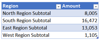
So, let’s just confirm what we are talking about. We’ve stored the region in cell B7 as shown below.

Now, we’d like to write a formula in C7 that retrieves the corresponding amount from Table1, shown below.
So, we start off with something like this:
=VLOOKUP(B7, Table1, 2, FALSE)
And, we hit enter, and get #N/A as shown below.
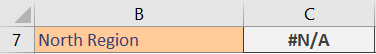
After reflecting on this, it makes sense. It makes sense because we used FALSE (or 0) for the 4th argument. That tells VLOOKUP to perform an exact match. Since “North Region” in B7 doesn’t match exactly to “North Region Subtotal” found in the table, we get an error. We discussed this long ago in Hack 3.
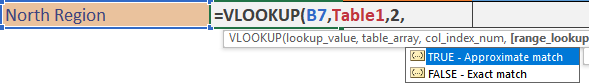
But, we know that the 4th argument has two possible choices. TRUE is described as Approximate Match, as shown below.
So, we give that a try. Drats! Same error, as shown below.
Ah, but then we remember something about the sort order mattering. We discussed this a while back in Hack 1.
So, we sort the table in ascending order by the first column. As shown below.
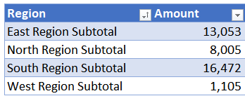
When we inspect our formula, it actually returns the value for the East Region, as shown below.

Yikes! What is going on here? Well, as we discussed in Hack 2, when we set the 4th argument to TRUE, we are really asking Excel to perform a range lookup. When VLOOKUP performs a range lookup, it scans down the first column. It returns the row where the table value is greater than or equal to the row and less than the value in the next row. While this makes perfect sense to us when the range is made up of numbers, it is a little harder to visualize when our lookup column has text values. But, effectively, the text string “North Region” is actually less than “North Region Subtotal” so the value from the East Region Subtotal row is returned.
So, it seems like we don’t want an Exact match. And, we don’t want an Approximate match. But, these are the only two choices for the 4th argument. TRUE or FALSE. There isn’t a third option. So, what are we supposed to do? Do it manually? No…of course not! That brings us to the hack.
Hack
What we are really after is a partial match. A partial match is where only part of the text needs to match. In this case, we want the lookup value “North Region” to match to the row that begins with “North Region” even if it includes something after, like “Subtotal” or a bunch of extra spaces. For now, let’s think about it like this. We want to find a row in the lookup range that “Begins With” our lookup value. How do we do that? Here’s the hack.
Hack: use a wildcard in the 1st argument
A wildcard is a character that can stand in to represent other characters. For example, the asterisk * can stand in to represent any number of characters. So, we need to join our lookup value to the asterisk. And, to do that, we’ll need an assist from the concatenation operator we discussed in Hack 7. The asterisk needs to be enclosed in quotes, so, our updated formula looks like this:
=VLOOKUP(B7&"*", Table1, 2, FALSE)
Now when we hit Enter … yes, it works!

Using the wildcard, we are asking VLOOKUP to go find a value in the lookup column that begins with the value in B7.
We could also search for a row that ends with the value in B7 like this:
“*”&B7
And, we could search for a row that contains the value in B7 like this:
“*”&B7&”*”
The sample file below contains the formulas in case you’d like to check them out.
If you have any other related VLOOKUP hacks, please share by posting a comment below!
- Sample file: VLOOKUP Hack 9.xlsx
Excel is not what it used to be.
You need the Excel Proficiency Roadmap now. Includes 6 steps for a successful journey, 3 things to avoid, and weekly Excel tips.
Want to learn Excel?
Our training programs start at $29 and will help you learn Excel quickly.
Thank you for this hack! I’ve wanted to do this before and ended up doing something much more cumbersome. Also, thank you for providing the written narrative. The company I work for doesn’t allow us to access YouTube, so the narratives are all I can use and your hints have been very helpful! Keep up the great work.
Thanks Traci, and I love this hack too 🙂
Oh my gosh, this is so helpful! Thank you! I have been going through a lot longer process just to get “subtotal” out of my vlookup. This way is so much easier! You just made my day.
Yay … happy to help 🙂
Great hack, thank you very much!
I need help with MS Excel. I have a long list of Bank Account transactions. I would like to code every single item. I don’t want to type anything, I want to upload a chart of account in a spreadsheet and want to fill every single cell selecting item from chart of Account
Anybody can help me with that ?
Sounds like a mapping table may be able to assist … more on that here:
https://www.excel-university.com/articles/journal-of-acct/the-power-of-mapping/
Hope it helps!
Thanks
Jeff
Hi Jeff, very useful. Is there a way to do this in reverse – where your lookup table contains a substring of your source table?
I have the exact same situation! Has anyone found a solution they can share?
I am trying to do the reverse as well. My best shot is this vba script.
you can use it with INDEX(ARRAY; MyMatch(lookup_value; lookup_array);col_num).
It actually works, but i would like to find a way with out the VBA script.
“Function MyMatch(lookup_value, lookup_array)
res = “”#N/A””
For i = 1 To Len(lookup_value)
For j = 1 To lookup_array.Rows.Count
substr = Left(lookup_value, i)
If substr = lookup_array(j) Then
res = j
End If
Next j
Next i
MyMatch = res
End Function”
Regarding “Hack: use a wildcard in the 1st argument”, what if the name of the region was john north vs just north. How would I use wild card to modify =VLOOKUP(“* “&B7&” *”,Table3,2,FALSE)
I’m trying to do something similar. For me, my “purpose” would read Subtotal North Region, or Subtotal Northern region, and my ‘data’ would say north.
Thanks in advanced.
Well explained Jeff, but I think it has character limitation upto 255. Formula is not working when I try more than that.
Thanks,
Cheera
Well explained Jeff, but I think it has the character limitation upto 255. Formula is not working when I try more than that.
Thanks,
Cheera
Hi All,
In fact excel shared provides actual differences between Exact, Approximate & Hack. I did not know it is not like the way as it looks.
I have a challenge in other way. I have data set where need to lookup from starts with.
Example: AmexIN01 = result should be ABCD
AmexIN* = ABCD
AmexUS=XYZ
Basically data may have some * which needs to be checked by formula and give result matching from Left.
Thanks in Advance
RC
i am trying this hack but is not working =VLOOKUP($E2&”*”,$A$1:$B$9,2,FALSE)
yes, same for me. It is not working.
Thanks for sharing
🙂
I have the same case, please post if we have any way to get it in reverse. It’s my daily activity and fed up with Right and Left formula.
Hi jeff thanks a lot it worked!!