VLOOKUP Hack #5: Different Tables
We are right in the middle of a blog series called VLOOKUP Hacks. We started by exploring the 4th VLOOKUP argument. Then we hacked the 3rd argument. Now, as you may have imagined, it is time to hack the 2rd argument. In this post, we’ll allow the user to retrieve values from different lookup tables.

Objective
Before we get too far, let’s be clear about the goal. The goal is to write a VLOOKUP function that will retrieve a value from a table that the user specifies. That is, there are a bunch of different lookup tables, and we want VLOOKUP to retrieve a value from whichever table the user identifies. I’ve created a short video demonstration as well as a written narrative for reference.
Video Demonstration
Narrative
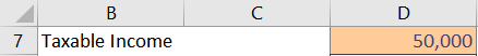
We would like to be able to enter a taxable income amount into a cell, and have Excel compute the correct tax amount. In order to compute the tax amount, we need to know a few things. For starters, we need to know the taxable income. So, we create a little input cell (D7) to store the taxable income, as shown below.
Then, we need to know the tax rates. We get the tax rates from the IRS and enter them into a table (named Single), as shown below.

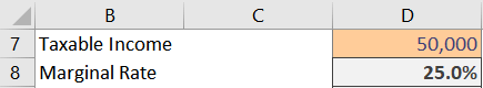
We’ll need to retrieve several values from the table in order to compute the correct tax amount. Let’s start by retrieving the marginal tax rate. The tax rate is in the 2nd column within the table (named Single), so, we write the following formula.
=VLOOKUP(D7,Single,2,TRUE)
When we inspect the formula result in D8, we confirm it returns 25% when taxable income is 50,000, so we are off to a great start, as shown below.
The VLOOKUP function retrieves the rate from the Single table. But, we know that the IRS creates separate tax tables for each filing status. So, we create one table for each filing status, as shown below.

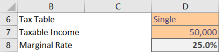
These tables are named Single, MFJ, HH, and MFS. Now, we just need to allow the user to identify the correct filing status table. So, we quickly update our workbook, and add an input cell D6 to allow the user to enter the desired table name, as shown below.
Now, we just need to update our formula to refer to the tax table input cell D6 instead of the table name. So, we just update the 2nd argument accordingly:
=VLOOKUP(D7,D6,2,TRUE)
But, drats! We get an error, as shown below.

So, apparently, VLOOKUP doesn’t allow us to identify the table name. Or…does it?
That brings us to the hack.
Hack
We can specify the lookup table, but, we need an assist from another function. So, here is the hack.
Hack: Use INDIRECT as the 2nd argument
The INDIRECT function converts a text value, such as “Single” in D6, into a valid Excel reference. That is, it will convert the text string “Single” into the corresponding table name Single. We update our formula by wrapping the INDIRECT function around the input cell D6 reference, as shown below:
=VLOOKUP(D7,INDIRECT(D6),2,TRUE)
And, yes…it works!
Now that we’ve got that part working, we can finish out the tax calculation as follows.
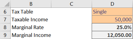
The next step is to compute the marginal income that will be taxed at the marginal rate. In theory, this is done by taking the taxable income amount (eg, 50,000) and then subtracting the beginning amount of the corresponding tax bracket (eg, 37,950).
Fortunately, we discussed how to retrieve the beginning point of a range in a previous post by using 1 as the 3rd argument. So, the formula would be something like this:
=D7-VLOOKUP(D7,INDIRECT(D6),1,TRUE)
The results are shown in D9 below.
We can then compute the marginal tax by multiplying the marginal income by the marginal rate. And finally, we need to retrieve the amount from the Plus column (so that we can add it to the marginal tax amount) with the following formula:
=VLOOKUP(D7,INDIRECT(D6),3,TRUE)
We add the retrieved amount to the marginal tax, and we have the Total Tax amount, as shown below.
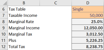
With the formulas complete, we are now able to easily enter the taxable income and tax table into the input cells, and Excel computes the corresponding tax. Nice!
Of course, we could combine all of these parts into a single formula, and, provide an in-cell drop down with data validation for the user to select the table. The sample file includes these enhancements in case you’d like to check them out.
If you have any other VLOOKUP hacks, please share by posting a comment below.
Excel is not what it used to be.
You need the Excel Proficiency Roadmap now. Includes 6 steps for a successful journey, 3 things to avoid, and weekly Excel tips.
Want to learn Excel?
Our training programs start at $29 and will help you learn Excel quickly.
Thanks for tips Jeff! Excellent.
Welcome 🙂
Hi Jeff, I am finding these VLOOKUP Hacks extremely interesting and see a distinct need to include them in my excel expertise.
This need may not arise immediately and dread the thought of trying to rack my brains to remember how exactly you went about explaining the procedure. Is there not a VLOOKUP Hacks note book that one could download and store for future reference purposes.
Hi Jon! Thanks I’m glad you are enjoying these posts. I plan to leave these posts online going forward for reference, but, I will be announcing a free e-book of them in a couple of weeks 🙂
Stay tuned …
Thanks
Jeff
Nice Hacks regarding VLookUp. Easy to follow and understand
I also really enjoy your posts . FYI – Webpage has a typo. After the picture of your ” drats” error showing the #n/a the spelling should be apparently .
Thanks for your kind note, and for pointing out that typo. I’ve fixed it now 🙂
Thanks
Jeff
SWEEEEET!
Hello Jeff. I have been following your presentations for sometime now and they are awesome. I really love them, and aside the knowledge you impart, you spice them up with your sense of humor. I am learning a lot of tips from you and just wanna say thank you.
Thanks for your kind note … I really appreciate it 🙂
Thanks
Jeff
What a great series, thank you for sharing all this information. I just watched all five, after re-reviewing your Power Query webinar and I’m putting these tips to work in a big annoying spreadsheet so IT can do the work instead of me! You do such a great job explaining these hacks that it’s easy to apply them. Thank you, Jeff!
Thanks Jeff Lenning for sharing all this. I also really enjoy your posts.
Thanks 🙂