Split Column Headers from Values
I was recently asked how to separate multiple column headers from their values. My favorite tool for transforming data like this is Power Query. So, this post walks through the steps with Power Query. Thanks Ron for your question!
Objective
Before we get into the steps, let’s visualize the start and end points. Ron states that the data combines each header and value in the same cell separated by a colon. I imagine it looks a bit like this:

Next, Ron asks how to remove the colon in each cell, place the headers in row 1, and place the values in row 2. I image the end result should look something like this:

The good news is that Power Query can help us with this. Let’s get to it.
Steps
We’ll perform these steps:
- Get data
- Transform data
- Load data
Let’s just jump right in.
Get data
First we need to get the data into Power Query. To do so, we head to the Data > Get Data command. Since our data is already in Excel, we select From Table/Range.
Note: if your data was somewhere else you’d pick the corresponding source option.
We are then presented with the following Create Table dialog, which is basically asking us to confirm the conversion of our data from an ordinary range to a Table.

Since our data doesn’t have a header row, we leave the My table has headers box clear and click OK.
We see our data in the Power Query editor, like this:

With this step complete, it is time to perform our transformations.
Transform data
The transformations we’ll perform are split, transpose, and promote. Let’s take them one at a time.
Split
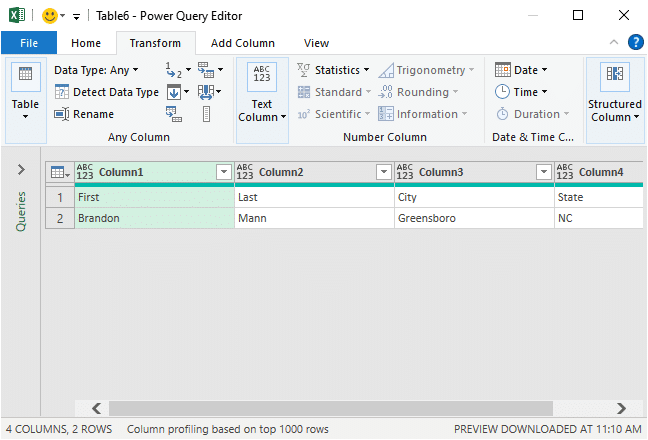
The first thing we’ll tackle is splitting the column headers (First, Last, City, and State) from their values (Brandon, Mann, Greensboro, NC). We right-click the Column1 header and select Split Column > By Delimiter. The following dialog appears, where we can confirm the default options or make any changes needed.

In our case, the defaults are fine so we just click OK
We see the results immediately in the editor:

Transpose
Next, we click the Transform > Transpose command, and bam:
Promote
Finally, we need to move the header labels into the header row. We click Transform > Use First Row as Headers, and bam:

With the transformations complete, it is time to load the data back into Excel.
Load data
We send the data back to Excel by clicking the Home > Close & Load To command, and opt to send it back to a Table … bam:
Yay … we did it!
Conclusion
The benefit of this approach is that we do not need to manually enter the column headers, they are automatically derived from the data. Plus, this query can be refreshed at anytime by right-clicking the results table and selecting Refresh.
Hope it helps … and thanks Ron for your question.
Sample file
Excel is not what it used to be.
You need the Excel Proficiency Roadmap now. Includes 6 steps for a successful journey, 3 things to avoid, and weekly Excel tips.
Want to learn Excel?
Our training programs start at $29 and will help you learn Excel quickly.
As usual, your approach is methodical and explanations are clear!
Just one follow up question. This post showed how to deal with a single instance of this data for Brandon Mann. I imagine there is a Mary Smith, John Public, and a thousand more that are structured exactly the same way, maybe in the same table or maybe in different forms. For the first case you want to extract the header information to create the table but in all the following records you would only want to extract the names. How would attach that?
Interesting: How would this be changed if all of your data was in this format?
First:Brandon
Last:Mann
City:Gainsborough
State:NC
First:Fred
Last:Bloggs
City:New York
State:NY
First:Bilbo
Last:Baggins
City:Miami
State:FL
This seems like a good solution when dealing with a single form that for some reason has brought in the label data along with the entered data.
On the other hand, correcting the problem further upstream would be preferable. Worst case, if the data can’t bec separated from the labels, It might be possible to create a template using an RPA tool like UiPATH and then “scraping” the data from each form at it’s source.
Your tutorials are so helpful and easy to follow!
Thanks!
Your tutorials are nothing short of spectacular.
Thanks for the posts!
Thank you 🙂
Hi Jeff. Some commenters above want a solution for more than one block of data or one that can react to additional data being added vertically. My solution is:
Source
Split Column by Delimiter
Remove Columns (Column1.1)
Add Index (from 0)
Add Modulo (value 4)
Add Subtraction (Index minus Modulo)
Remove Column (Index)
Pivoted Column (pivot on Modulo, values from Column1.2, Don’t Aggregate)
Remove Column (Subtraction)
Rename Columns (First, Last, City, State)
Close and Load
M-Code from Advanced Editor is shown below. This will work to unstack more than one record and or adding records and refreshing the query with each subsequent record showing in the appropriate First, Last, City and State columns. I hope this is useful to someone. Thanks for the challenge and inspiration to learn. Thumbs up!!
let
Source = Excel.CurrentWorkbook(){[Name=”Data”]}[Content],
#”Split Column by Delimiter” = Table.SplitColumn(Source, “Column1”, Splitter.SplitTextByEachDelimiter({“:”}, QuoteStyle.Csv, false), {“Column1.1”, “Column1.2″}),
#”Removed Columns” = Table.RemoveColumns(#”Split Column by Delimiter”,{“Column1.1″}),
#”Added Index” = Table.AddIndexColumn(#”Removed Columns”, “Index”, 0, 1, Int64.Type),
#”Inserted Modulo” = Table.AddColumn(#”Added Index”, “Modulo”, each Number.Mod([Index], 4), type number),
#”Inserted Subtraction” = Table.AddColumn(#”Inserted Modulo”, “Subtraction”, each [Index] – [Modulo], type number),
#”Removed Columns1″ = Table.RemoveColumns(#”Inserted Subtraction”,{“Index”}),
#”Pivoted Column” = Table.Pivot(Table.TransformColumnTypes(#”Removed Columns1″, {{“Modulo”, type text}}, “en-US”), List.Distinct(Table.TransformColumnTypes(#”Removed Columns1″, {{“Modulo”, type text}}, “en-US”)[Modulo]), “Modulo”, “Column1.2″),
#”Removed Columns2″ = Table.RemoveColumns(#”Pivoted Column”,{“Subtraction”}),
#”Renamed Columns” = Table.RenameColumns(#”Removed Columns2″,{{“0”, “First”}, {“1”, “Last”}, {“2”, “City”}, {“3”, “State”}})
in
#”Renamed Columns”
Thank you!!
Jeff, very nice explanation and to the point!
You could always go back to good old Text to columns & Index.
Slightly simplified version of Wayne’s multi-data blocks solution:
Source
Split Column by Delimiter
Added Index
Integer-Divided Column
Pivoted Column
Remove Other Columns
Basically we are going to add an index column, then transform the index column using Integer Divide, then pivot based on the column that contains your desired column headers (your transformed index column provides you with an anchor column; note, if you have varying amounts of data in your blocks you will want to Add a Conditional Column and at each instance of the primary data point you return the number from the index column, otherwise return null, then fill down; this will create an anchor column so you can then pivot).
let
Source = Excel.CurrentWorkbook(){[Name=”Table6″]}[Content],
#”Split Column by Delimiter” = Table.SplitColumn(Source, “Column1”, Splitter.SplitTextByDelimiter(“:”, QuoteStyle.Csv), {“Column1.1”, “Column1.2″}),
#”Added Index” = Table.AddIndexColumn(#”Split Column by Delimiter”, “Index”, 0, 1, Int64.Type),
#”Integer-Divided Column” = Table.TransformColumns(#”Added Index”, {{“Index”, each Number.IntegerDivide(_, 4), Int64.Type}}),
#”Pivoted Column” = Table.Pivot(#”Integer-Divided Column”, List.Distinct(#”Integer-Divided Column”[Column1.1]), “Column1.1”, “Column1.2″),
#”Removed Other Columns” = Table.SelectColumns(#”Pivoted Column”,{“First”, “Last”, “City”, “State”})
in
#”Removed Other Columns”