Sort by Color

In this post, I’ll answer a question submitted by reader Chérie about sorting by color. The basic question is this. “I have created a color coded list, where yes=green, no=red, maybe=orange, and other is any other color. How can I sort the list so that all the yes rows are first, then no, then maybe, and then other?”  Thanks for your question! Time to get to work.

Objective

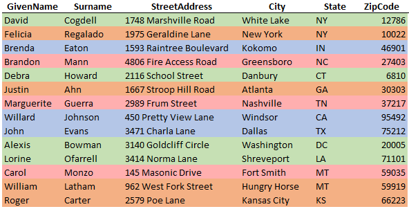
Let’s be clear about our objective. There are two ways to identify rows. One is by using a cell value and the other is with cell formatting. For example, if the rows are identified by color only, and there is no corresponding cell value, the list may look like this.

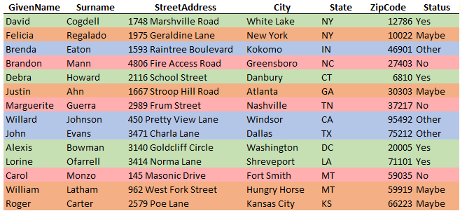
But, additionally, there may be a cell value involved with the identification, as illustrated by the Status column below.

Now, let’s sort both types of lists in a specific order: yes, no, maybe, and other.

Sort by Color

First, we’ll sort by color, which works on both types of lists. To sort the list by color, add Sort and Filter controls by selecting any cell in the range and then the following Ribbon command:

• Data > Filter

This will provide little drop-downs on the header row as shown below.

Expand any of the drop-downs and select the following:

• Sort by Color > Custom Sort

This opens the Sort dialog. In the Sort by field, pick any column that includes the colors. Then, choose to Sort On Cell Color. Pick the color you want to appear at the top of the list. Then click the Add Level button, and repeat using the next color, and so on. When you are done, your dialog should look something like this.

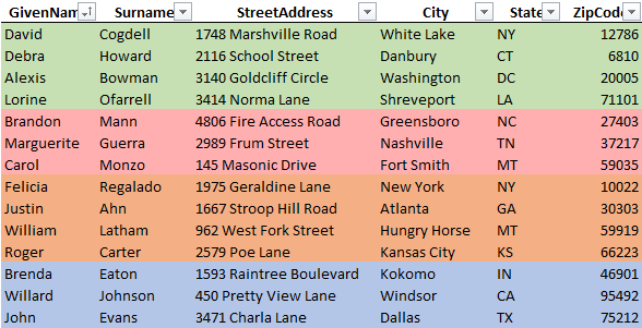
Apply the sort and your list should now appear in the desired order, as shown below.

When you have a cell value, we can optionally use a custom list. Let’s check that out.

Custom List

When you have a column that contains cell values, but the desired sort order is other than ascending or descending, you can create a custom list. For example, consider the data below.

Let’s say we tried to sort by the Status column values. If we used an ascending sort, we’d end up with Maybe, No, Other, Yes. If we used descending, we’d end up with Yes, Other, No, Maybe. Neither of these built-in sort orders are what we want, which is Yes, No, Maybe, Other. This is when a custom list can come in handy. To create a custom list, open the Options dialog with the following command.

• File > Options

Click the Advanced category, and then scroll way down until you see a button named Edit Custom Lists as shown below.

Click it to open the Custom Lists dialog. Simply enter your list entries in order, Yes, No, Maybe, Other, and then click Add. This will create a new custom list, as shown below.

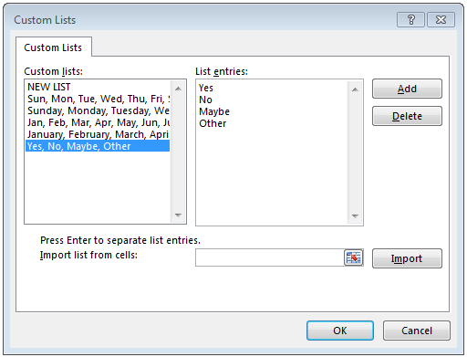
Now, this custom list will be available in other workbooks and various places within Excel, including PivotTables, Fill Series, and in the Sort dialog.

To sort our data using the order of the custom list, simply select any data cell and then the following Ribbon command:

• Data > Sort

This opens the familiar Sort dialog, and this time, we’ll ask Excel to Sort by the Status column. In the Order drop-down, select Custom List, and then pick your fancy new custom list. The Sort dialog will look something like this.

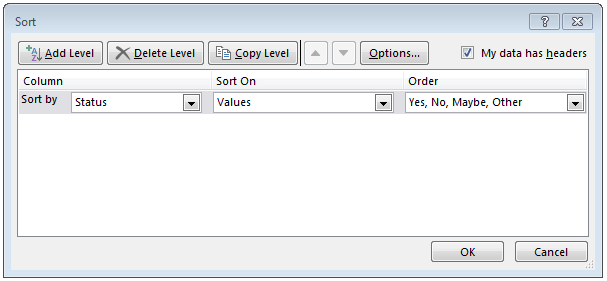
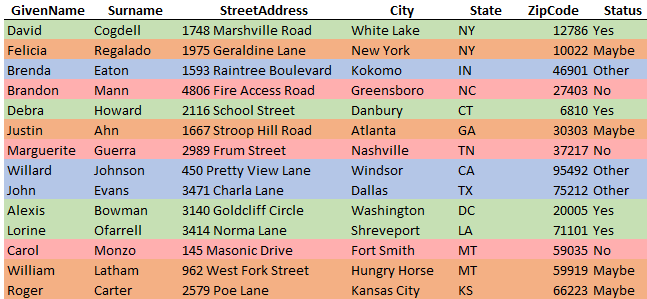
Apply the sort and bam…custom sort order applied!

Objective accomplished!

If you have any other sorting tips, please share by posting a comment below…thanks!

Additional Resources

Sample Excel file: SortByColor