Pivot Text Values with Power Query
In this post, we’ll talk about how to Pivot text values with Power Query. We would like to do this even if there are a variable number of fields per record. This can be REALLY hard to visualize based on a short text description, so I think it is best to show screenshots of the before and after. Let’s just jump right in.
Objective
We have data that looks like this (before):
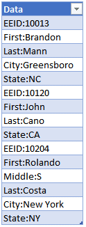
Let’s observe a couple of things:
- Not all fields are included for each employee. For example, some employees have a City field, and some don’t. Thus, our solution needs to work even when there are a variable number of fields (First, Last, City) per record (per Employee).
- Even though all employees do not contain all fields, all field labels are consistent. The State field is always called State and not something else, like Region.
- Each employee has a unique identifier that isn’t duplicated with other employees. In our case, it is the employee id (EEID) field. This unique key field can be numeric or text, it doesn’t matter in our solution.
- The EEID is the first field for each employee … other fields can appear in any order.
We want to make it look like this (after):

Now that we see where the data is coming from and where it needs to go, let’s see how we can get it there with Power Query.
Video
Walkthrough
We’ll walk through the steps as follows:
- Get data
- Transform data
- Load data
Let’s do this thing.
Get data
First we need to get the data. In this case, the data is in an Excel table, so we use the Data > Get Data > From Table/Range command.
This gets the data and we can see a preview in the Power Query Editor, like this:
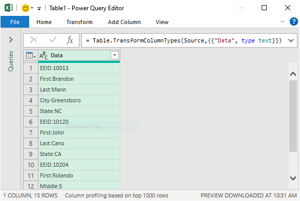
Note: If your data was somewhere else, you’d use the corresponding Get Data option.
With the data in Power Query, we can now perform a few transformations and get it into our desired format.
Transform data
In summary, we will perform the following transformations:
- Split Column by Delimiter
- Change Headers
- ID Column
- Fill Down
- Pivot
Let’s go one by one.
Split Column by Delimiter
Since the Labels and Values are stored in the same column, we’ll split them into their own columns. We notice they are separated by a colon, so we use the Transform > Split Column > By Delimiter command. The Split Column by Delimiter dialog appears:

Power Query guessed Colon correctly, but if it guessed incorrectly you can easily change the delimiter. We click OK and bam:

Change Headers
Although this step isn’t strictly necessary, it makes the following steps more clear. So, we will change Data.1 to Label, and Data.2 to Value. You can easily rename the header labels by double-clicking the header, typing the desired header, and hitting Enter on your keyboard.
Now we look like this:

ID Column
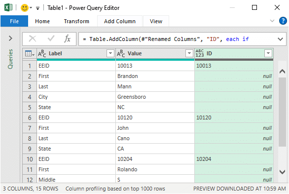
Next, we need to create a column that contains just the employee ids (EEID value).
One way to do this is to use the Add Column > Conditional Column command. In the resulting Add Conditional Column dialog, we give our new column a name such as ID (don’t use the same value as the EEID data label). Then, we update the dialog to use this logic: If the Label column value Equals EEID Then the output should be set to the Value column. It looks like this:

We click OK and bam:
Fill Down
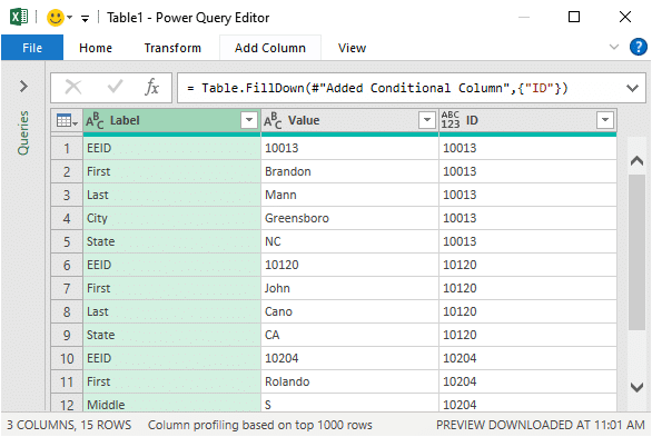
We want each row in the ID column to have the ID value. To accomplish this, we’ll select the ID column and use the Transform > Fill Down command. Bam:

And now, we are ready for the best transformation yet … the Pivot!
Pivot
At this point, we want to basically ask Power Query to create one new column for each unique value in the Label column. That is, new columns for EEID, First, Last, City, and so on. So, Power Query will use the values in the Label field to create the new column headers. Then, we’ll ask Power Query to place the corresponding Value into each new column. Power Query knows which fields belong together by the ID column.
The first step is to select the column that contains the new column headers, in our case the Label column like this:
Next, we click the Transform > Pivot Column command. In the resulting Pivot Column dialog, we confirm that it will use the names in the Label column to create the new columns. We set the Values Column to Value. Next, we need to expand the Advanced options and select Don’t Aggregate. It looks like this:

When we click OK … magic!
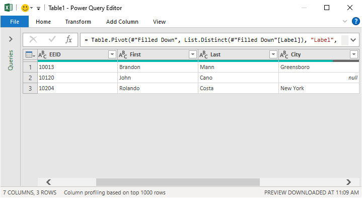
We can optionally delete the ID column, and we are ready to send the results back into Excel.
Load data
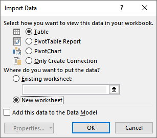
We click the Home > Close and Load To command, and we opt to send the data into a Table in a new or existing worksheet:
And got it:

Yay … we did it!
Power Query is such an amazing tool, and I hope this post helps you use it more effectively.
If you have any thoughts, suggestions, or questions, please enter a comment below … thanks!
Sample file
Excel is not what it used to be.
You need the Excel Proficiency Roadmap now. Includes 6 steps for a successful journey, 3 things to avoid, and weekly Excel tips.
Want to learn Excel?
Our training programs start at $29 and will help you learn Excel quickly.

The vedio was amazing. I have watched excel training by many experts Jeff Lenning by far is the best. He has a way of breaking the steps into small steps and give little very important tips as he does that for example in the video above he just said Power Query is case sensetive and continues…
I love his teaching methods and he always pleasantly smiles as he shares his knowledge.
Thanks Marsy 🙂
Hi Jeff,
Thanks for the great detail explanation and screenshots. I tested it creating the same data and it worked like a charm.
One question I have is can you explain why the requirement for the Additional Conditional Column? I tested without adding this column and the fill down and as you probably expect, I received an error. Trying to understand so I can apply this to my own live examples.
Will the conditional column always be the first line? What determines the column to use?
Thanks!
Rachel
Hi Rachel!
We need the ID column so that PQ knows which rows belong together. So I think of it as a ‘group by’ column. Hope this helps … thanks!
Thanks
Jeff
Ahh ok makes sense.
Thank you.
Rachel
🙂
That is magic indeed, particularly if you have ever tried to program table manipulations like these.
Thanks Jimmy!
Jeff, I am devoted follower. Thank you for keeping me in the “know”!
Excellent! My job requires me to get data in a usable format for end-users, and PowerPivot & PowerQuery are making my job so much easier. Your training methods are exceptional, and I like it that you provide written instructions (and lots of screenshots – yay!) along with a video as I can’t always watch videos at work. Two thumbs up!
Thanks!
You always do a great job of picking useful, real-world examples and giving clear explanation of the solution and the thinking behind it.
Thanks!
🙂