List of Worksheets in a Drop Down
In this post, I’ll answer a question I received from Sara about how to create a drop down with each worksheet name and reference it in a formula to retrieve values from the selected sheet. As this is Excel, there are a variety of alternatives to accomplish this. In this post, I’ll demonstrate one such solution that uses a defined name, data validation, and the INDIRECT function. Plus, as a bonus, I’ll demonstrate how we can dynamically generate the list of sheet names using Power Query. Thanks Sara for your question!
Video
Objective
First, let’s be clear about what we are trying to accomplish. We have a workbook with multiple sheets … perhaps one sheet for each department like this:
![]()
Each sheet has the same basic data structure, like this:

On a summary sheet, we want to create a drop down so a user can pick one of the department sheets, like this:
And when a sheet is selected, we want to use the selected sheet name in a formula to reference values on the selected sheet, like this:
So, let’s get to it.
Walkthrough
Overall, here is the game plan:
- Step 1: Create a table with the sheet names
- Step 2: Create a defined name that references the table name
- Step 3: Create a drop down with data validation
- Step 4: Use the INDIRECT function to create a reference to the selected sheet
- Bonus Step: Optionally, use Power Query to create the list of sheet names dynamically
Step 1: Create a Table with the Sheet Names
Let’s start by creating a table with the sheet names. If there are only a few sheets, creating the table manually is the easiest. If you have a ton of sheets, be sure to check out the final Bonus step which demonstrates how to use Power Query to create the list of sheet names dynamically.
Begin by typing the sheet names into some cells, like this:
Then, convert that ordinary range into a table by selecting it and selecting the Insert > Table command. The resulting table should look something like this:
If this is the first table in the workbook, it probably has a name of Table1. You can view or edit the table name as desired by using the Table Design > Table Name field.
Step 2: Create a Defined Name
Next, we want to create a Defined Name that we can use in the next step. To do so, just click Formulas > Name Manager.
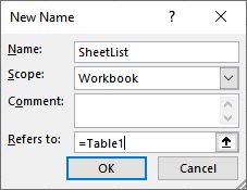
In the resulting Name Manager dialog, click New and then create a new name such as SheetList and set it equal to the table name in the previous step (eg, =Table1), like this:
Note: the equal sign = in front of the table name is required.
Step 3: Create a Drop Down
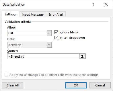
Now we can create the drop down. Select the cell for your drop down, and select Data > Data Validation. In the resulting Data Validation dialog, you want to Allow a List, and the Source is =SheetList (or whatever name you defined in the previous step), like this:
Note: the equal sign = in front of the SheetList name is required.
When you click OK, you should have a functioning drop down, like this:
Next, we want to reference the selected sheet name in our formula. To do that, we’ll want to use the INDIRECT function.
Step 4: Use INDIRECT
The INDIRECT function converts a text value into an actual Excel reference.
Let’s get warmed up with a simple example of a cell reference. We could pass a text string “A1” into the INDIRECT function and it would return an actual reference to cell A1. This formula would look like this:
=INDIRECT("A1")
Let’s take the next step and figure out how to reference a cell on another sheet. If we type an equal sign = into any cell, and then click a cell on a different worksheet, we can inspect the resulting reference to see how Excel does this.
For example, the reference to cell A1 on a sheet named Dept A looks like this:
='Dept A'!A1
Two things to note:
- First, we use an exclamation point ! between the sheet name and the cell reference
- Second, we enclose the sheet name in single quotes
So, let’s put this all together.
The desired sheet name is selected from a drop down. Let’s say that drop down is in cell C5, like this:
And let’s say we want to retrieve the Manager from the selected sheet, which is stored in B4, like this:
We would then write a formula using INDIRECT, like this:
=INDIRECT(" ' " & C5 & " '!B4 ")
Note: I added a bunch of extra spaces and some underlines to try to make it easier to read. These spaces should be removed from your actual formula.
Let’s understand what is going on. First, we use INDIRECT to convert a text value into an actual Excel reference.
The text value includes three components, all joined together with the concatenation operator &:
- The opening single quote (enclosed in quotes) for the sheet name
- The reference to the drop down cell (which has the sheet name)
- The closing single quote for the sheet name, then the exclamation point to separate the sheet name from the cell reference, and finally the desired cell reference (enclosed in quotes)
When we hit Enter, the formula retrieves the value from B4 from the sheet selected in the drop down … yay!
What if we wanted to sum an entire column from the selected sheet? No worries. We can essentially use the INDIRECT function in formulas where we would use a normal cell or range reference.
So, to sum the entire C column on the selected sheet, we write a formula like this:
=SUM( INDIRECT("'" & C5 & "'!C:C") )
Note: I added extra spaces to try to make the formula easier to read.
Bonus Step: Use Power Query to create a Dynamic Sheet List
When there are only a handful of sheet names, typing them in manually is the fastest and simplest. But, what if you have a ton of sheet names, or you are adding or removing sheets frequently from the workbook. In this case, we can have Power Query generate the list of sheet names for us.
One way to do this is to click Get Data > From File > From Workbook from the Get & Transform command group. Next, we browse to the workbook. In the resulting Navigator dialog, we just pick any sheet (it doesn’t matter which one at this point because we will change it later).
Next we click the Transform Data button to open the Power Query Editor.
We use the X to delete all applied steps except for the Source step. So, at first the Applied Steps list may look something like this:
Then, click the X to delete all but the Source step:
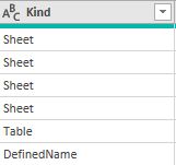
At this point, you will see a list of any Sheets, Tables, and Defined Names that are in the workbook. These are identified in the Kind column:
Since we only want to return a list of Sheets, we filter the Kind column to keep Sheet rows only.
Note: even if you have only Sheet rows, you still want to apply a Text Filter = Sheet so that new tables or names that are created later will be excluded.
At this point, we should see a list of the worksheets in the Name column:
Since we want to exclude the Summary sheet from the drop down, we’ll just use a filter to exclude it.
Also, we only want to return the Name column to Excel, so, we right-click the Name column header and select Remove Other Columns.
Next, we click Close & Load To … and select Table. We can insert the table into either a new or existing sheet as desired.
The resulting table should look like this:
Now, to tell the drop down to reference this new table instead of the original table (blue), we go back to the Name Manager (Formulas > Name Manager). We Edit the SheetList name and change it to reflect the Power Query results table (green). You can determine the name of the table by clicking it and looking at the Table Design > Table Name field.
Once done, we can safely delete the original table (blue) from the workbook.
Going forward, when we change sheet names, add new sheets, or remove sheets, we can (1) Save the workbook and then (2) right-click the Power Query results table (green) and Refresh. This will populate the results table with the current sheets, and the drop down will reflect them. Yay … we did it!
NOTE: you will need to Save the workbook for any changes in the sheet names to be reflected. In other words, when you Refresh the table, Power Query looks at the saved version and excludes any changes that have been made since you last saved.
NOTE: if you didn’t filter for type Sheet as suggested, your list of sheet names may include table names and defined names over time as they are added, including the results table. If this happens, you can edit the query and apply a filter to include only Kind=Sheet.
NOTE: if you rename or move the location of this workbook, you’ll want to edit the query’s Source step to reference the new name or location.
Conclusion
If you have any improvements or other approaches to this, please share by posting a comment below … thanks!
Sample file: SheetDropDown.xlsx
Excel is not what it used to be.
You need the Excel Proficiency Roadmap now. Includes 6 steps for a successful journey, 3 things to avoid, and weekly Excel tips.
Want to learn Excel?
Our training programs start at $29 and will help you learn Excel quickly.


Really enjoyed this!
I love this, I have wanted to do this for years, INDIRECT is such a gem!
Thanks Jeff!
Nice tutorial. In the past I’ve used a different method to create a dynamic list of sheet names, but this works quite elegantly.
I was trying to use the Power Query method to create a list of worksheets but I seem to run in to an issue when I try to reference the same workbook where I am creating the list as Excel tells me that the workbook is being used by another process i.e. because the workbook is open. Is it only possible to create an index of worksheets using Power Query if the list exists in a separate workbook or am I doing something wrong?
Is there a way to create a hyperlink to the respective sheet when it is selected from the dropdown menu? Rather than retrieving data from that sheet, I would like to be able to use the dropdown menu to navigate to any sheet in the workbook.
Awesome tricks, thank you so much.
This tutorial gave me the answer to the exact two problems I was trying to solve. Awesome!!!
Just a question though. I have several sheets I don’t want to include in the drop down within the Power Query, so I excluded them as shown above with the Summary sheet. However, whenever I add a new sheet it does not appear automatically (after save and refresh), so I need to go back and add it within the Power Query. Does Power Query allows only one exclusion in order to automatically add new sheets? Or is there another solution to my issue?
Thanks a lot in advance
Is there a way to make a second dropdown list based on the first? I created a dropdown based on the sheets I have in the workbook but want a second dropdown that shows the cells from the sheet selected in the first dropdown.
This is an amazing method! I’d trying to keep track of monthly evaluations for my job and managing the tabs gets cumbersome. This is the perfect solution. However, it doesn’t work for me. I’m getting the same error that Stuart was having in another comment. Workbook is being used by another process. My workbook is hosted on Sharepoint, but it downloads a local copy to my OneDrive folder where I should be able to point the query to. Doesn’t work. Is this due to the nature of Sharepoint or OneDrive interfering? How can we get around this issue?