Indirectly Refer to Table Columns
Previously, we explored using the INDIRECT function to refer to various tables in a workbook. In this follow-up post, we’ll expand the discussion and refer to individual table columns.
Objective
Let’s start with our objective. We have several tables in a workbook. They have the same structure and store department data. For example, here is the Department A table.
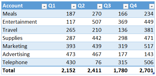
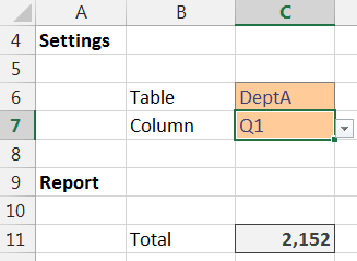
We would like to be able to select the table AND the column from drop-down controls, and have Excel use the selected table and column in a simple SUM function as illustrated below.
Alright, let’s get to it.
Structured Table References
First up, let’s figure out how Excel’s structured table references work. A Structured Table Reference (STR) allows us to refer to a specific area within a table, such as a specific column. STRs begin with the table’s name followed by the specific area enclosed in square brackets [].
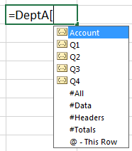
Referencing a specific column is accomplished like this: TableName[ColumnName]. For example, to refer to the Q1 column in the DeptA table, we would use: DeptA[Q1].
In addition to referring to specific columns, we can refer to specific rows. For example, to refer to just the header row of the DeptA table, we could use DeptA[#Headers]. To get a list of the available STRs, type the table’s name in a formula and then type the open square bracket. Excel will display a list of valid STRs in the auto-complete list, as shown below.
Now that we know the anatomy of STRs, let’s move on to the drop-down cells.
Data Validation
To create the drop-down controls, we’ll use the data validation feature.
The drop-down control in C6 is generated with the Data Validation feature by allowing a list equal to the table names. Setting this up was discussed in the previous post.
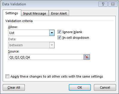
The drop-down control in C7 is generated with the Data Validation feature by allowing a list equal to the column names. To do so, select the input cell C7 and then the Data Validation ribbon command. Set it to allow a list equal to the column labels you’d like to be displayed, as shown below.
INDIRECT
At this point, all that remains is to write the formula. We need to create the desired reference with a text string and then pass it to the INDIRECT function. The INDIRECT function will convert the text string into a valid Excel reference.
For example, let’s say that we ultimately wanted to sum up the Q1 column of the DeptA table. We could use the following formula.
=SUM(DeptA[Q1])
But, rather than entering the STR directly into the formula, we want to store the table name in cell C6 and the column name in C7. So, we would build the STR using the concatenation operator (&), as follows:
=C6 & "[" & C7 & "]"
Note: spaces are shown in the formula above to make it easier to read.
Assuming DeptA is stored in C6 and Q1 is stored in C7, the formula above returns the desired STR, DeptA[Q1].
To convert the STR into a valid Excel reference, we’ll use the INDIRECT function, as follows.
=INDIRECT(C6&"["&C7&"]")
Finally, we’ll sum the cells in the reference with the SUM function, as follows.
=SUM(INDIRECT(C6&"["&C7&"]"))
This will compute the sum for the selected table and column, as illustrated below.
If you have any additional ideas or methods, please share by posting a comment below!
Additional Resources
- Sample Excel File: IndirectTableColRef
- Dynamically reference table columns with INDEX/MATCH: SUMIFS with Dynamic Table data
- Related post: Referring to Tables Indirectly
- Note: our tables had the same column headers; if they were different, you could use Data Validation and allow a list equal to =INDIRECT(C6&”[#Headers]”) so that the column drop-down would provide the column headers found in the table identified in C6
Excel is not what it used to be.
You need the Excel Proficiency Roadmap now. Includes 6 steps for a successful journey, 3 things to avoid, and weekly Excel tips.
Want to learn Excel?
Our training programs start at $29 and will help you learn Excel quickly.
I’m using your approach to create dynamic features built into a dashboard. I’m attempting to make the STR [column specifier] be determined based on the output of a form control….. without success. Will this approach work with other formulas such as SUMPRODUCT.
Barry,
Yes, the INDIRECT function should work in functions where a typical range reference is expected.
Also, to SUM based on a dynamic column reference, have a look at this post as well:
https://www.excel-university.com/use-the-column-header-to-retrieve-values-from-an-excel-table/
Hope it helps!
Thanks
Jeff
I am trying to do something slightly different but similar to the above. It seems like I should be able to use index/match but I can’t get it to work. Do you have any suggestions? I want to create a conditional lookup based on something like the following table:
Product Name
Fruit Apple
Fruit Pear
Veg Carrot
Veg Leek
What I would like to do is create a conditional lookup so that if someone types Fruit into cell A1, then the dropdown on cell B1 only shows the options Apple and Pear. I know I can do this by creating a table for Fruit and another table for Veg but I would like to keep all the data in a single table. The reason for this is the actual problem I am solving is more complex than my example with 4 columns ie 4 levels of data. Any suggestions would be gratefully received.
Ian
Hey Ian
Mr. Jeff wrote a blog on exactly this:) Here’s the link https://www.excel-university.com/create-depdendent-drop-downs-conditional-data-validation/
Let me know how that works,
Kurt LeBlanc
I’ve spent several evenings trying to figure out how to convince Excel that my chosen dropdown value needed to be read as a columnheader, so I could create a second dropdown based on that column. Without any previous knowledge of Excel and the proper terminology it has been extremely difficult to figure out.
This bit “So, we would build the STR using the concatenation operator (&), as follows:” finally got me my solution. THANK YOU SO MUCH!
🙂
Hello,
I’ve build a spreadsheet containing one master data table with one column per month and one student name per individual row in the first column. The month‘s headers are named using thé twelve months names. There are twelve additionnal tabsheets, named as well using the same months names.
My goal is to retrieve the student‘s hours per month stored in each monthly tabsheet, and to report them into the master data table.
I succeeded doing the job using a vlookup and an indirect function which takes the header string into account in order to search into the relevant tabsheet., i.e., INDIRECT(J$1), where J1 contrains „April“ for example.
To make it more robust, I would like to use the [#Headers] and [#This Column] instead of the hard coded cell reference.
Would you know which syntax to use for such a purpose?
Within the table, to refer to the header cell within a column, you should be able to use the following:
=Table1[#Headers]
When I test it here, it returns the corresponding column label correctly for each table column.
Hope this helps,
Jeff
Hello,
I use this formula to calculate weeks cover of inventory:
=SUM(DD19:DD22)*U19/T19*4
The sum function calculates how many units of a product remain in inventory. Each line contains the inventory values for a specific product. In many cases, there are several lines with inventory values for the same product and those values must be summed to capture all the inventory of that item.
Each week the column where the sum function is calculating the current inventory of an item changes because 4 new columns of data are added, representing the inventory activity during the week.
So each week, I update all of the weeks cover formulas with a new column name so that the sum function calculates from the correct column which contains the latest inventory values.
For example, next week the weeks cover equation for a certain item with 3 lines of inventory values will be =SUM(DH19:DH22)*U19/T19*4
The next week that line function would be =SUM(DL19:DL22)*U19/T19*4
Since it is tedious to update the column name for the sum portion of the weeks cover calculation for each line, i would like to use an independent cell that the weeks cover function references in order to define the column where the inventory values will be summed.
Perhaps the new weeks cover item would be
=SUM(VARIABLE19:VARIABLE22)*U19/T19*4
When the cell containing the VARIABLE is updated, all of the formulas with that contain that variable would update. That way, I could define the column where the sum calculation is performed for numerous line items by updating the cell containing the variable.
I would like to update one cell per week, and all of the weeks cover calculations would be updated with the correct column name instead of the direct column name that I manually update each week.
Can this be done with excel?
Thanks!