Income Tax Formula

In this post, we’ll examine a couple of ideas for computing income tax in Excel using tax tables. Specifically, we’ll use VLOOKUP with a helper column, we’ll remove the helper column with SUMPRODUCT, and then we’ll use data validation and the INDIRECT function to make it easy to pick the desired tax table, such as single or married filing joint.

Objective

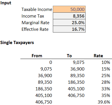
Before we get ahead of ourselves, let’s be clear about our objective. We want to store a tax table in Excel. We want to enter a taxable income and have Excel compute the tax amount, the marginal tax rate, and the effective tax rate. This idea is illustrated in the screenshot below.

Since this is Excel, there are many ways to achieve the goal. In this post, we’ll use VLOOKUP with a helper column, we’ll then eliminate the helper column with SUMPRODUCT, and then we’ll allow the user to select the correct tax table with INDIRECT. Let’s explore each approach.

VLOOKUP

The VLOOKUP function is a traditional lookup function that returns a related value from a lookup table.

Since the VLOOKUP function returns a single value, and not an aggregated sum of many values, we’ll need to modify our tax table by adding a helper column. The helper column will compute the cumulative tax for each tax bracket, as shown below.

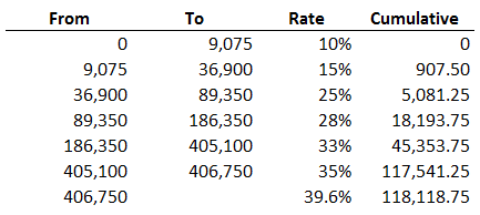
The cumulative helper column formula is straightforward, we simply apply the marginal rate to the bracket income. The sample file below contains the formula for reference.

If we assume a taxable income of $50,000, we need to write a formula that basically performs the following math:

=5081.25+((50000-36900)*.25)

We can use VLOOKUP to obtain all of the related values from the tax table based on the taxable income. The basic syntax of the VLOOKUP function follows:

VLOOKUP(lookup_value, table_array, col_index_num, [range_lookup])

Where:

• lookup_value is the value we are seeking
• table_array is where we are looking
• col_index_num is the column that has the value to return
• [range_lookup] will be TRUE since we are performing a range lookup, not seeking an exact matching value

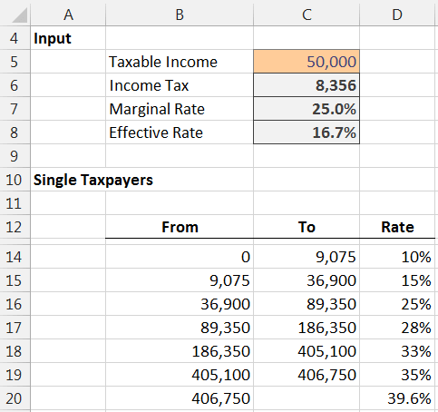
Let’s apply the VLOOKUP to the tax calculator below.

We’ll substitute each table value in the following formula with a VLOOKUP function:

=5081.25+((50000-36900)*.25)

Doing so produces the following formula:

=VLOOKUP(C5,B13:E19,4,TRUE)+(C5-VLOOKUP(C5,B13:E19,1,TRUE))*VLOOKUP(C5,B13:E19,3,TRUE)

Now, we can enter a taxable income into C5 and our formula applies the desired math.

But, what if we did not want our worksheet to contain the cumulative tax amount helper column? We can use the SUMPRODUCT function instead.

SUMPRODUCT

The SUMPRODUCT function is able to return the sum of multiple products. That is, it is able to apply the rate to each bracket and return the sum. This capability eliminates the need for a helper column.

This function is trickier to visualize because it operates on multiple cells at once.

For our discussion, let’s consider the updated calculator in the screenshot below, which contains no helper column.

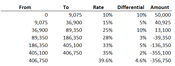
If the taxable income was $50,000, we would like Excel to perform the following math. It needs to multiply all $50,000 by 10% because all $50,000 is taxed by at least 10%. To that, we need Excel to add 5% of 40,925 (50,000-9,075), because the differential rate of the next bracket is 5% (15%-10%). To that, we need to add 10% of 13,100 (50,000-36,900), because the differential rate of that bracket is 10% (25%-15%).

The differential rate idea is illustrated in the screenshot below.

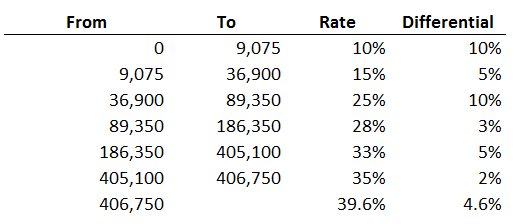
Using the differential rate instead of the marginal rate simplifies our SUMPRODUCT function.

To visualize the math, we could set up a new column that shows the amount to be applied to each differential rate by subtracting $50,000 from each income bracket, as shown below.

To see the extended tax, let’s add another column that computes the amount by the differential rate, shown below.

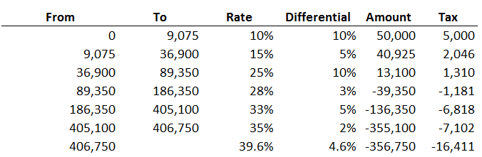
But, we only want to include the tax rows that are positive numbers. We could add another column that converts the negative values to zero, and then add it up, as shown below.

Fortunately, $8,356 is the same value returned by our VLOOKUP formula, so, I think our math is good.

With the basic idea in mind, let’s reconsider the following worksheet.

Since our goal is to eliminate helper columns, we can ask the SUMPRODUCT function to compute the differential rate, compute the amount to apply to each rate, and exclude negative values all in a single function:

=SUMPRODUCT(D14:D20-D13:D19,C5-B14:B20,N(C5>B14:B20))

The SUMPRODUCT function returns the sum of the product of its arguments. That is, it multiplies its arguments together, and then computes the sum. Let’s walk through the arguments. The first argument, D14:D20-D13:D19, computes the differential rate. (Note that D13 needs to be an empty cell, not a text string, which is why we made row 13 skinny.) The second argument, C5-B14:B20, computes the amount to apply to each differential rate. The third argument, N(C5>B14:B20), excludes negative values by converting the boolean result of the comparison, eg, TRUE or FALSE, to 1 or 0. When Excel multiplies the row by 0 it is excluded from the sum.

Illustration

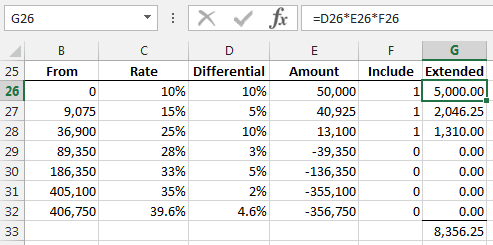
I’ll set up some new formulas in another area of the worksheet to illustrate the math that is performed by SUMPRODUCT. Note that the cell references below are different than the ones above. SUMPRODUCT uses columns B and C. To illustrate the logic, I set up column D to represent the first argument (differential rate), column E to represent the second argument (amount), and column F to represent the third argument (TRUE/FALSE logic to include or exclude the row). Column G multiplies these columns, and G33 provides the sum.

If your goal is to eliminate helper formulas, SUMPRODUCT can be helpful. However, my preferred approach is to use VLOOKUP and INDIRECT as demonstrated next.

VLOOKUP and INDIRECT

We want to provide the user with the ability to select a filing status, such as single or MFJ. We’ll store rates for each filing status in a separate Excel table (Insert > Table). We’ll name each table with the desired filing status. We’ll use data validation to provide an in-cell drop down with the list of choices. We’ll use the VLOOKUP approach demonstrated above to retrieve related values and compute the taxable income. We’ll use the INDIRECT function to tell Excel which table to use for the lookup. Whew…that’s a lot of moving parts. Since they have been explored previously in this blog, rather than provide each of the steps here, I’ll simply provide references to the related blog posts in the additional resources list below.

Here is our final product:

All approaches discussed above are included in the sample file below. Please feel free to check out the file as needed.

If you have any alternative approaches, please share by posting a comment below…thanks!

Additional Resources

• Sample file: Tax
• VLOOKUP posts
• INDIRECT posts
• Data Validation posts
• Table posts
• Thanks to Don Steele for sharing his marginal tax rate Excel file: marginaltaxrate