Four Ways to Select Every Other Row in Excel

Selecting every other row in Excel can be helpful. Aside from making it easy to get rid of duplicate rows, it can also be a great way to highlight important information, make the data easier to read with formatting, and more.
However … if you’ve ever tried to select every other row in Excel, you know that there’s no straightforward way to do so. Here are four easy (and quick) ways to do it with a bit of guidance for when to use each method!
1. Use the Ctrl button to manually select rows
If your worksheet doesn’t have many rows, holding down the Ctrl key on your keyboard while selecting the desired rows in your spreadsheet is probably the simplest way to select every other row.
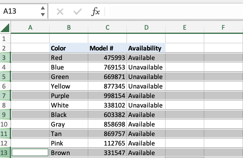
When you click on the row number, the entire row will be highlighted. You can then hold down the Ctrl key and continue to select additional rows. This type of cell selection is called a non-contiguous range.
While it’s easy, it isn’t necessarily practical if you have lots of rows. Manually selecting rows can take a lot of time and leaves room for error. If you have many rows, the remaining options may be a better fit.
2. Format alternating rows with a Table
If your goal is to have a different format for alternating rows for cosmetic purposes, or to make your data easier to read, then a table is an easy option.
1. Select any cell in your data range.
2. Select Insert > Table
3. Excel will apply a default format, which includes a different format for alternating rows.
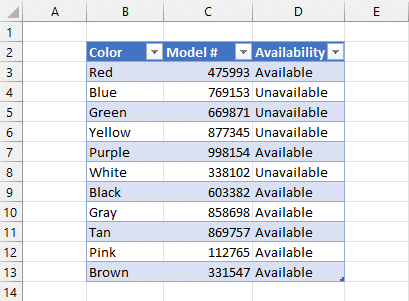
This option is called Banded Rows, and you can toggle that on/off by using the Table Design > Banded Rows checkbox.
You can also select various table styles by using the Table Design > Table Styles gallery.
3. Use a helper column with the Go-To Special command
If your goal is to delete every other row, a helper column that uses alternating values is a good option. You can see an example of such a helper column in the screenshot below.
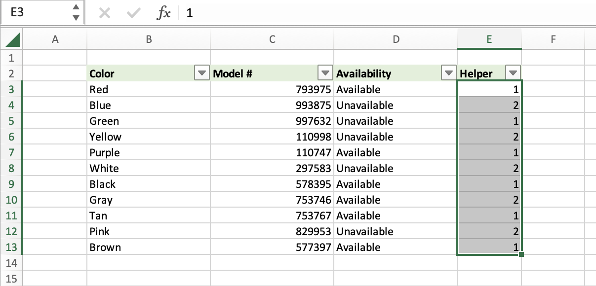
1. Prepare a helper column that alternates between two different values. In the above example, every other row in the helper column contains the number 1 or 2. You can also use the fill handle to speed up the process of filling the alternating values down. Enter the first two values, 1 and 2, and then select those cells. Hold down the Ctrl key and drag the fill handle down. Excel will repeat 1 and 2 all the way down.
2. Select the first cell in the helper column and then extend the selection all the way down the column.
3. On the Home ribbon item, click Find & Select, then Go-To Special, and choose Column Differences.
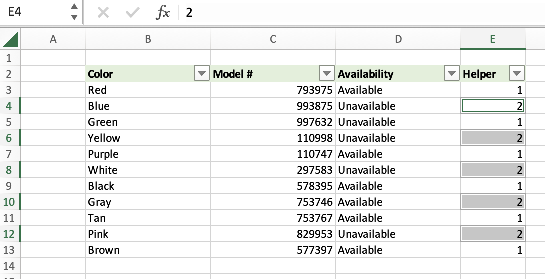
This will select all values in the column that are different than the active cell, which is typically the first cell you click when you drag to select an entire range. (You can press Tab to move the active cell within a selected range.)
Once every other cell in that column is selected, you can right-click any of the selected cells and select Delete. In the resulting dialog, select Entire row to delete every other row in your dataset.
4. Use filters to select every other row in Excel
If you want to select the entire row (instead of just the helper column cells as in the previous option), this method will work well. Excel’s ability to filter rows is useful when you want to view certain sections of data, but it also provides a quick way to select every other row.
1. Just as you did in the example above, prepare a helper column that alternates between two different values.
2. Select the entire range, go to the Data ribbon item, and click the Filter button.
3. Choose a filter for the helper column that shows the alternating rows you’d like to select.
4. If you want your selection to include only the data cells, select the entire filtered range. If you want your selection to include the entire row, select all rows that span the filtered data. Selecting filtered rows (or cells) actually selects both the visible and the hidden rows.
5. Click Go-To Special and select the Visible cells only.
This will change the selection to include only the rows that are showing, and deselect the hidden/filtered rows.
You can then click the Filter control (drop-down) for the helper column (the one with the active filter) and clear the filter for that specific column. Now, every other row should be selected.
Note: don’t remove the filter controls by clicking Data > Filter or the Data > Clear buttons. Instead, select the filter control (the little drop-down) for the helper column and clear that specific column filter.
Bonus: select the entire row with VBA
As a bonus, here is a snippet of VBA code you can swipe to select every other row.
1. Select any span of rows.
2. Open the VBA Editor using the shortcut Alt + F11. Select New Module, and copy/paste this code:
Sub AlternateRows()
  Dim Rng As Range
  r_start = Selection.Row
  r_end = Selection.Rows.Count + r_start - 1
  Set Rng = Rows(r_start)
  r_start = r_start + 2
  For r = r_start To r_end Step 2
    Set Rng = Union(Rng, Rows(r))
  Next r
  Rng.Select
End Sub
Note that it’s always a good idea to back up your work and test VBA code before applying them to important Excel files. VBA is powerful, so you don’t want to risk messing up your workbooks.
3. Select View, then Macros, and Run.
This will select every other row within the original selected range.
If you want to more practice with VBA, check out our post on Microsoft Excel macros to learn about recording macros, editing VBA codes, and running them in Excel.
Do you have any other quick ways to select every other row in Excel? Let us know in the comments!
Excel is not what it used to be.
You need the Excel Proficiency Roadmap now. Includes 6 steps for a successful journey, 3 things to avoid, and weekly Excel tips.
Want to learn Excel?
Our training programs start at $29 and will help you learn Excel quickly.
I don’t know if this tip necessarily fits with your theme, but I use conditional formatting to highlight every other row. This formula can be easily modified to highlight evens, odds, or multiples.
Highlight the range of cells that you want to apply banding and use this rule:
MOD(ROW(),2)=0
Even rows: ISEVEN9ROW())
Odd rows: isodd(row())
I hope this proves to be useful.
This is great, thank you for sharing 🙂
Agreed. This is how I highlight alternate rows, as well. What I see the most from beginner to mid-level Excel users is that conditional formatting is woefully underutilized.
For dynamic row reports, you can add value checks so that only rows with data in a particular column are highlighted. For example, applying the following conditional format to 50 rows where only 10 rows currently have data and Column A is the determination for highlighting
=AND(LEN($A1)>0,MOD(ROW(),2)=0)
will result in rows 2, 4, 6, 8, and 10 to be highlighted but the remaining rows will have no highlighting. However, when you add more data in additional rows, the highlighting will automatically take effect on the additional rows.
Changing the formula to
=AND(LEN($A1)>0,MOD(ROW(),2)0)
will highlight rows 1, 3, 5, 7 and 9.
Using conditional formatting is nothing more than having an understanding of what makes something TRUE or FALSE.
I noticed that my post had a typo: Even rows: ISEVEN9ROW()), should be ISEVEN(ROW()). Excel – endless possibilities.